Contributed by Arda Kosar, Kyle Szela, Hayes Cozart and Radhey Shyam . They are currently in the NYC Data Science Academy 12 week full time Data Science Bootcamp program taking place between January 11th to April 1st, 2016. This post is based on their fourth class project - Machine learning (due on the 8th week of the program).

OUTLINE

• Part I. Introduction
• Part II. Ideas & Methods
• Part III.Models
  • Part III-I.Logistic Regression
  • Part III-II.Support Vector Machines
  • Part III-III.Adaptive Boosting
  • Part III-IV.Neural Networks
  • Part III-V.Random Forests
  • Part III-VI.XGBoost, Stacking and Ensembing

Part I. Introduction

The Higgs Boson is a landmark discovery that will help us to understand the basic nature of the universe. It was discovered first by the ATLAS experiment at the Large Hadron Collider, CERN in 2012. The Higg’s Boson decays into two tau particles giving rise to a small signal buried in background noise. The goal of the Higgs Boson Machine Learning Challenge was to classify the characterizing events detected by ATLAS into "tau tau decay of a Higgs boson" versus "background."

First step was to analyze the data and look for missingness in the data. We found that the missing columns have some interesting patterns and they depend on the columns “PRI_jet_column”, which is the number of jets having integer values of 0,1,2, or 3 where larger values have been capped at 3.

The Jets are the experimental signatures of quarks and gluons produced in high-energy processes such as head-on proton-proton collisions.

For PRI_jet_column=0, there were 10 columns having NULL values (-999), these are the columns which describe the Jet when it is equal to 0. For example, “DER_mass_jet_jet”, the invariant mass (20) of the two jets (undefined if PRI jet num ≤ 1).So, it does not make sense to take into account the attributes of the jet(s), since they don't exist.

For “PRI_jet_column” = 1, there were 7 columns having NULL values and they describe the jets when their number is 2, So we deleted these 7 columns.

For “PRI_jet_column” = 2 or 3, we did not delete any columns.

Full list of deleted columns:

“PRI_jet_column” =0: DER_deltaeta_jet_jet, DER_mass_jet_jet, DER_prodeta_jet_jet, DER_lep_eta_centrality, PRI_jet_leading_pt PRI_jet_leading_eta, PRI_jet_leading_phi, PRI_jet_subleading_pt,PRI_jet_subleading_eta, PRI_jet_subleading_phi

“PRI_jet_column” =1: :DER_deltaeta_jet_jet, DER_mass_jet_jet, DER_prodeta_jet_jet, DER_lep_eta_centrality, PRI_jet_subleading_pt, PRI_jet_subleading_eta, PRI_jet_subleading_phi

We divided the training data into three groups depending on the value of “PRI_jet_column”
1. “PRI_jet_column” =0
2. “PRI_jet_column” =1
3. “PRI_jet_column” = 2 or 3

Additionally, we deleted PRI_jet_column as it is constant in three groups and will not help in predicting in any machine learning algorithms after dividing the training data in three groups.

Part II. Ideas & Methods

The two main methods of feature engineering we used in this project were capturing the missingness in the dataset. The first method used was counting the NA's in the data set and then grouping by the number of NA's into different sets of the data. The second way this was done was through the variable that counted the number of jets. For this method, the data was separated into three separate groups based on whether it had a jet number of zero, a jet number of one, or a jet number of two or three. How these features were used will be explained further in the explanation of the models.

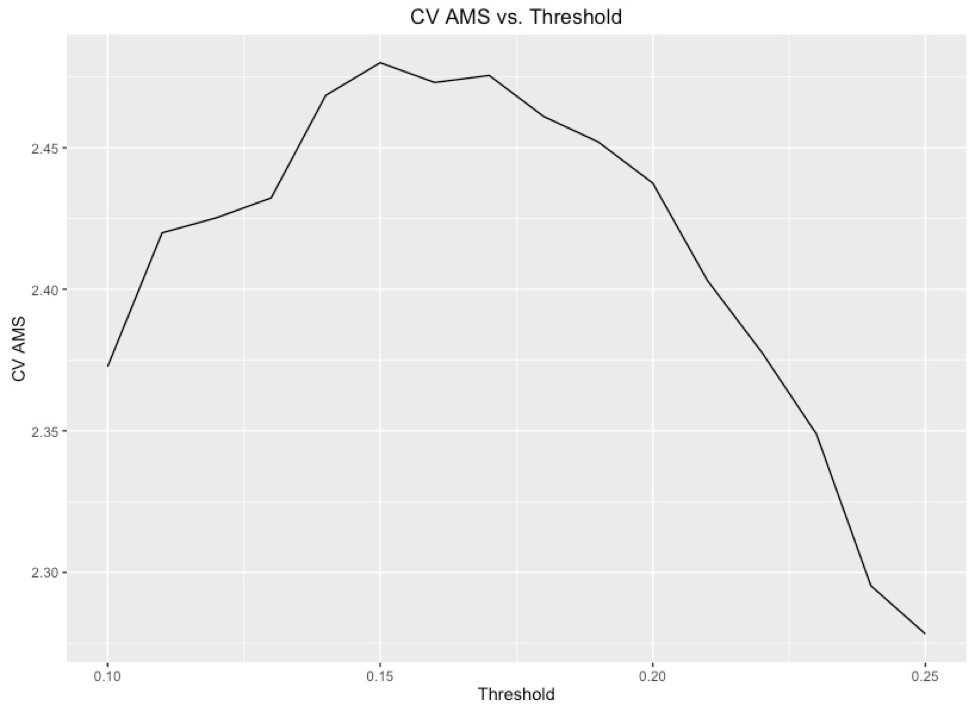
In this competition, the AMS penalized false positives more significantly than false negatives. To combat this issue of penalty, in this project, we utilized cross-fold validation to pinpoint where the perfect cutoff threshold was for signal particles to achieve a maximal AMS:

In order to submit to Kaggle for evaluation of our current model, we took the probabilistic predictions from the model and sorted them from most like a background signal (closest to 0) to most like a Higgs Boson signal (closest to 1). We then added rank order, as per the instructions of the competition and set 15% of the highest ranked signals to be Higgs Boson signals. In order to find this threshold, we took a single XGBoost model and found the AMS for each different percentage. As one can see, a threshold of 15% gives the highest AMS scored, and we correspondingly used this throughout the rest of our project to achieve results.Below is the work flow for our submissions:

Also, as a part of our EDA, we explored correlations among all the variables. We found that certain variables were highly correlated with others. This could be a potential problem for linear model analysis. Below is the correlation plot for the dataset:

Part III. Models

Part III-I. Logistic Regression

Since the scope of the competition is a classification problem, we started with logistic regression. We divided the training and test datasets into three categories based on Jet Number respectively. For each subgroup, we imputed any missing values with NAs and standardized variables by scaling data between 0 and 1 using normalization function. By performing a Chi Square testing on the full model, we saw that the P value of the overall test of deviance was high enough to indicate that the full model was a good overall fit.

We then proceed with principal component analysis for the training set. For the subgroup jet num=0 for example, we found that there were 7 major principal components:
PC1 was highly correlated with DER_mass_MMC, DER_mass_vis, DER_sum_pt, PRI_tau_pt
PC2 was highly correlated with DER_mass_transverse_met_lep, DER_pt_ratio_lep_tau, PRI_lep_pt
PC3 was highly correlated with DER_pt_h, DER_pt_tot
PC4 did not seem to be highly correlated with variables
PC5 was highly correlated with PRI_tau_eta, PRI_lep_eta
PC6 was highly correlated with PRI_tau_phi and was negatively correlated with PRI_lep_phi
PC7 was highly correlated with PRI_met_phi

For model selection, we chose to use AIC since the primary goal of our logistic regression was predictive rather than descriptive. By conducting forward selection AIC, we found that the best reduced model with the smallest AIC for jet num=0 is:
Label ~ DER_mass_transverse_met_lep + PRI_tau_pt + DER_deltar_tau_lep + DER_mass_vis + DER_sum_pt + DER_pt_ratio_lep_tau + PRI_met_sumet + PRI_met + DER_mass_MMC + PRI_lep_eta + PRI_met_phi

Given the correlation analysis we did, we also wanted to reduce correlations among variables in our model. We tried to remove a variable PRI_tau_pt, which was highly correlated with multiple variables in our model. As a result, although it reduced correlations, the deviance test rejected it since it didn’t provide sufficient information as well as our best model did. Also, the model yielded less prediction accuracy than our previous model. Thus we retained our best model.

We repeated previous steps for subgroup jet num=1 and jet num=2, 3. We combined prediction results, sorted them and ranked them to create an order. Then we set threshold to be 15%, the optimal threshold value we discovered through cross-validation. As a way to validate our model performance, we calculated the AMS and our logistic regression model got a score of 2.6.

Part III-II. Support Vector Machines

Regarding the support vector machines (svm) we first tried a support vector classifier, with linear kernel and cost =1 as default, in order to get a base reference for our svm model. However this model took more than 5 hours to complete and still did not finish, therefore, we terminated the process and thought of a new approach.

First we wanted to have an estimate of how long it takes to implement the svm model. We took 4% of the dataset, implemented our svm model and it trained in 51 seconds. We took 5% of the dataset, it trained in 98 seconds. We took 10% of the dataset and it took ~10 minutes to train. So we saw that the training time increases exponentially as we increase the amount of the data we were training on.

We also searched for the operational numbers regarding svm and we found that, in general terms, for 250000 data points it will require (250000^3) = 1.5625e+16 number of operations to implement the full model. If we create 20 folds and implement a model on each 5% it will require 3.90625e+13 number of operations which is 400 times less than implementing on the full model.

So we created 20 folds and implemented our svm on each 5%. Then we predicted with each model on the whole test set and we took row wise averages in order to get our final predictions. However this approach did not perform well with the AMS score = 1.76.

We wanted to implement a support vector machine, with a radial kernel. We tried to do a local cross-validation to tune for the parameters gamma and cost however the process took longer than 7-8 hours so we terminated the execution.

Part III-III. Adaptive Boosting

Another approach we took was, we implemented adaptive boosting model in order to see if it gave us a better result. We used R package called "ada" to implement this method. Package ada is used to fit stochastic boosting models for a binary response (Additive Logistic Regression: A Statistical View of Boosting by Friedman, et al. (2000)). Package applies adaboost procedures, which in the core is combining multiple weak classifiers in to one strong classifier. What adaboost helps is choosing the training set for each new classifier, depending on the result of the previous one. Also, it determines how much weight should be assigned to each classifiers' proposed answer when combining the results.

We carried out local cross-validation to find the best parameters, and mainly we focused on the shrinkage parameter (nu). Below is the local cross validation results graph for the nu parameter:

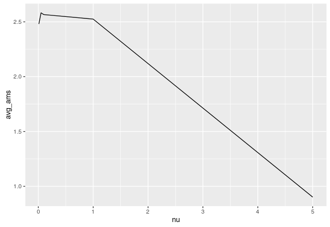
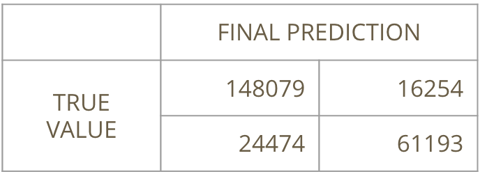
We implemented our model with our best nu. We also did some feature engineering in this model by adding the xgboost stack predictions as a new feature to the adaboost model, and the model overall scored an AMS = 3.68784, which was 127th on the leaderboard. Our prediction accuracy was 83%. Below is the confusion matrix of the final adaboost model:

Part III-IV. Neural Networks

We divided the Training data into three categories based on Jet Number.
We imputed any missing values with zero and scaled the data between 0 and 1 using normalize function (subtract the minimum value of columns and divide by the difference of minimum and maximum values).
We tried several libraries for neural network and finally used the “neuralnet” library in R because we can define a vector of integers specifying the number of hidden layers and neurons in each layer. Also, we used the Logistic function as the activation function and set Linear Output to False.

For single hidden layer, we tried different number of neurons in the range of 10 to 100. For neurons less than 20, accuracy was not significant and for neurons around 100 neurons it took more than 4 hours to converge and hence we could not try on all the three groups in training data set.

We also tried using three hidden layers and changing the number of neurons in each layers 10 to 100. For small number of neurons, the accuracy was not significant, when we increased the number of neurons to 100 in each layer, it took more than 6-8 hours for single group and neutral network algorithm did not converge, so we have to set “rep” =10, number of repetitions and it converged in 1 or 2 out of 10 attempts. So, due to lack of computational power and no set algorithms to tune parameters we did not get desired results for neural networks. Additionally, we think that we could have used some transformations for some columns or some feature engineering so that the neural networks could converge faster.

Part III-V. Random Forests

We started with the random forest trying to make a good baseline before we did any feature engineering. With this basic random forest that had all the defaults we got an AMS score of 2.904 without setting the threshold to 15%. After we set the threshold to 15% the AMS score jumped all the way up to 3.401 this would be the baseline to determine whether or not the features we added were increasing the AMS score.

The first piece of feature engineering was splitting the data into three, based on the variable PRI_jet_num. This variable was shown to account for all the missingness in the data set other than mass. The groups of the data were for Jet number 0, jet number 1, and jet number 2-3. Once we had split the data into three we ran a random forest on each subset of the data then recombined all the predictions they made at the end to create the submission file. This feature addition by itself moved the AMS score up to 3.407. We then used the out of bag error for the models and found the best mtry to use for each of the three random forests. For jet num 0 the best mtry was found to be 3, for jet num 1 the best mtry was found to be 12, and for jet num 2-3 the best mtry was found to be 7. One thing we found interesting was that the second group seemed to want to use almost half the variables while the other two were around the number of variables you would expect for the number of variables being used in each subset. One reason this might be is that the missingness in the data was due to information on the jets and you need at least 2 jets to get complete data. So we determined that what the random forest might be trying to do is when it only has information on one jet rather than two it could be trying to make sense of those numbers by randomly picking more variables.

Before we continue and describe the last feature engineering we did, we need to explain something weird that happened when we were creating the models. Early on in the process, when we were creating subsets, we forgot to drop all the NA columns from the subsets of the data. What meant by this is we did not drop the columns that had no information in them other than NA's. This created a problem for random forests as it randomly picks variables to split. This means that those constant columns are able to be chosen but will add no value to predicting whether the observation was a signal or background. However, a very strange thing happened when we removed these useless columns from the data set. The AMS score actually decreased, this literally did not make any sense at all. What we found out was that it was due to the seed we were using just randomly pulling worse for the better model, than the one with the useless columns. We tried out some other seeds and found that it was just a fluke that the AMS decreased for that one instance.

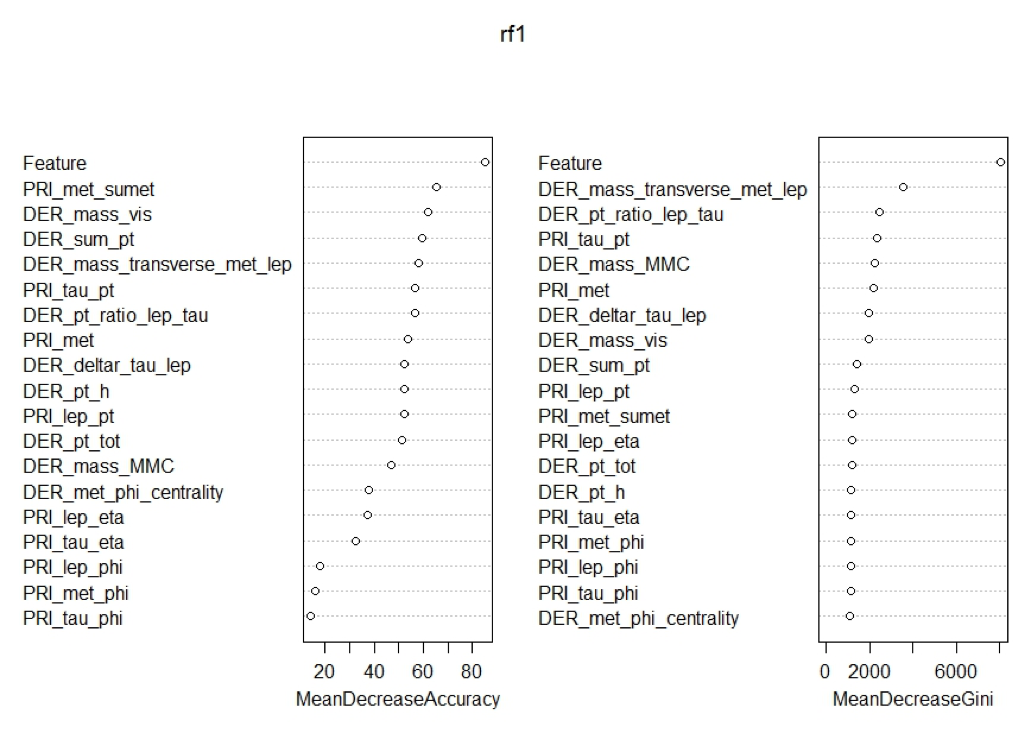
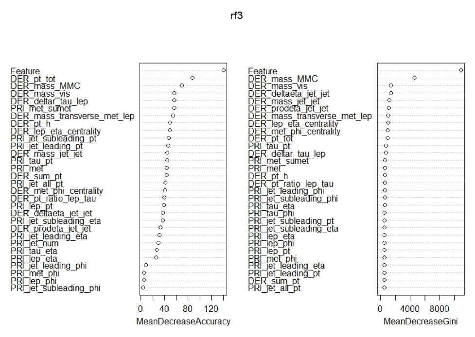
Now that we had cleaned the data of useless constant columns the final piece of feature engineering we did was adding the predictions of xgboost as a variable to both train and test sets. This final edition is what got us to the final AMS score of 3.469, though if we look at the variable importance charts below we see that there may have been some other feature engineering that we could have done dealing with the phi variable.

Part III-V-I. Variable Importance

In all three charts below we see two things shared no matter which subset of the data was used. First, we see that the added feature of xgboost was the most important feature for prediction found in all three random forest models. Second, we see that all the variables that end in phi are at the least important features for every model. This means that it may increase the prediction of the models if we removed them from the subsets as they do not seem to be adding much predictive value.

Part III-VI. XGBoost, Stacking and Ensembling

In order to explain the rest of our strategy and methods, we must first explain stacking. Through stacking, one can leverage the results of previous models predictions on the test and train set. In this case, we used 5-fold cross validation as is depicted in the image below. In cross validation, one splits the dataset into different parts, one part to train the model, and one part to test. This is useful because it can give us a relatively accurate estimate of what our error will be on the real test data. Additionally, in the case of stacking, instead of only testing on the portion of the train we use for cross validation, we also test on the entirety of the test set as well. Also, since in cross validation, each test fold is exclusive from the other folds, all of the predictions made on the folds are in aggregate predictions on the entirety of the train set. Through the saving of these predictions, we can add the new feature from the testing on the 5 folds of the train set as a new feature of the train set, and similarly, we can add our predictions on the test set (in our case we took the average across the 5 different predictions on the entire test set) as the corresponding new feature to the one in the training set.

The model that we used for stacking was XGBoost, but first we needed to optimize a single XGBoost in order to get our best predictions for subsequent stacking. Some early ideas to improve the cross validation score of this model were the separation of the datasets based on the number of NA’s. As noted above, there was a definitive pattern for the NA’s, so we thought that splitting the datasets based on this helped add valuable information for the model training to use in order to make predictions. In the end, though, when we compared the cross validation score between the XGBoost model using this splitting technique, and the same model using XGBoost parameters where we simply indicated the presence of NA’s, the simple solution provided a higher AMS score.
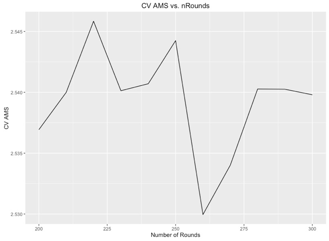
Additionally, we cross validated to find the best number of rounds for this model. We kept the learning rate at 0.1 eta because we felt that this learning rate was slow enough to capture the dataset, but lessening this would require us to increase the number of rounds necessary to achieve similar results. Additionally, we wanted to focus more on ensembling methods. Below is the graph of rounds versus cross validated AMS. Due to the volatility of the AMS, we implemented 2 fold cross validation across 3 different random seeds in order to acquire a good estimate of test error. The results shown (above and below for the threshold and the number of rounds) are the average AMS across all 6 models:

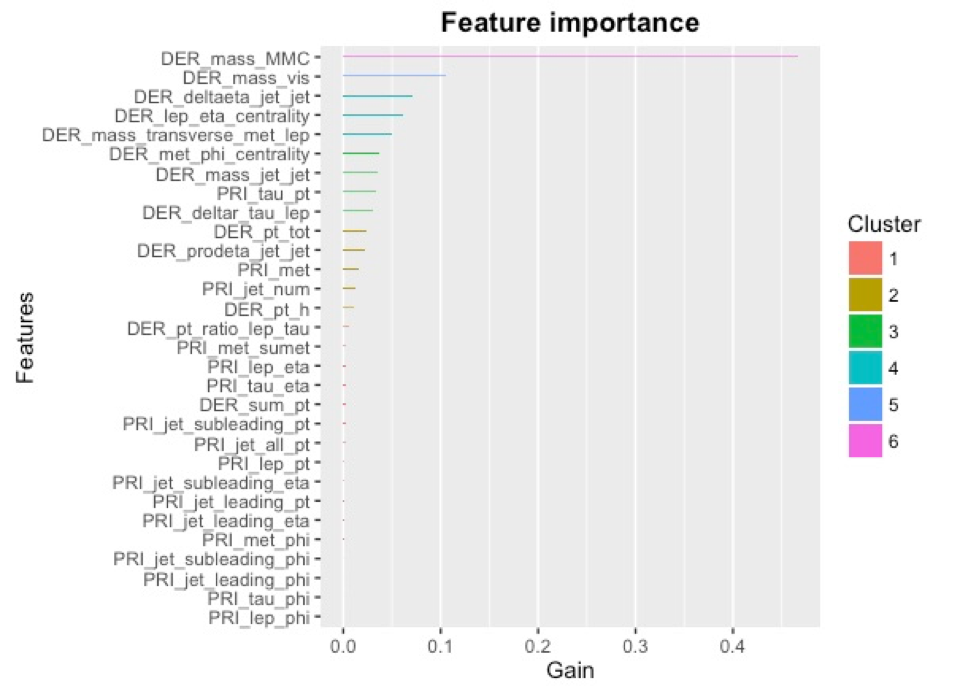
We had also come into this project with the intention of implementing feature engineering. In the case of XGBoost, we tried numerous different features, most to no avail. Each feature was tested utilizing 2 fold, 3 seed cross validation as noted above. Attempted features were summing the rows, the number of NA’s as a numeric feature, the number of NA’s as a factor feature, the number of jets as a factor, dropping the 5 lowest importance phi variables (as shown in the below graphs), and dropping jet_subleading_eta feature. Of these numerous attempts, the only improvement in cross validated AMS was dropping the 5 phi variable columns. The idea behind this was that these phi variables alone did not add any information to the model and may have caused overfitting. There may have been a possibility of creating features based on the differences of the phi variables, but we did not end up implementing these. Below is the variable importance plot for a single xgboost with no NA’s:

Lastly, we took all of the above models and created the ensemble depicted below. We implemented 3 different stacks at varying seeds and trained 3 different XGBoost models on the output of these stacks. The simple average of the predictions from these 3 XGBoost models was able to score a 3.729 AMS on the Private Leaderboard, which earned a ranking of 28th. We then took the average output from each stack for the training and testing sets and added them as new features for both Adaboost, which increased to an AMS of 3.688, giving a rank of 127th on the Private Leaderboard, and our Random Forest implementation, which achieved a score of 3.496 AMS on the Private Leaderboard for a rank of 823rd. We then used a weighted average of these three models to achieve a final AMS score of 3.734 with a final ranking of 26th.