Ames Housing Price Predictions - Model Ensembling
Introduction
The purpose of this project was to create an accurate model for Ames, Iowa home prices from the dates 2006 - 2010. This prediction model would learn from a Kaggle dataset (and competition that can be found here: https://www.kaggle.com/c/house-prices-advanced-regression-techniques). Originally, this dataset was made by a professor, Dean de Cock at Truman State University as a class project. This dataset has grown in popularity and now is the basis for a highly frequented Kaggle training competition. It has 79 explanatory features to help describe a house and the surrounding property ranging from square footage to more subjective or categorical features such as quality or garage type.
Our intrepid team of four set off to explore our dataset, draw inferences and ultimately create a model to predict the correct price of a home in Ames.
Contents:
- The Data:
- Explore dataset
- Look for trends
- Basic stats
- The Models
- Present models used
- Explore pros and cons of models
- The Pipeline
- Cleaned data --> base modeling --> metamodeling --> output csv
- Discuss code structure
- The Results
- Test set performance
- The Future
- How we could improve our approach to the problem
- What we could have done better
1. The Data
We have about 2900 observation total with 79 numeric and categorical features; split evenly between training and test datasets. Our output variable is sales price. There is some missing data, some outliers, and some skewed variables. We want to fix some of these problems before we can have strong models.
First, let us have a look at the distribution of the response variable, sale price. We can see from the figure that the distribution of sale price is right skewed. To fix this, we will perform a log transform on the sales price. The blue line represents the original skewed data distribution while the black line represents the transformed normal distribution. Next, we plotted boxplots and scatterplots to show sale price versus different features. For example, on this sale price versus neighborhood boxplot, it seems that there is a strong correlation between neighborhood and sale price.
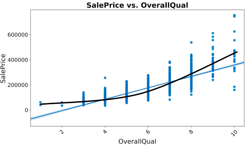
On the scatterplot of sale price versus overall quality, we have another strong correlation. However, when we take a closer look, the sale price actually increase exponentially as the overall quality increases.
On the correlation plot, we can see that first floor square feet is highly correlated with total basement square feet and garage cars is highly correlated with garage area. In the feature engineering, we will address these issues.
In addition to some of the EDA and transformations above, the team removed several high price outliers and added some features such as total livable square footage.
2. The Models
For the models, we chose a variety of different base models such as Lasso and Ridge regression, Elasticnet, deep XGBoost, shallow XGBoost, GBoost, LGBM, and Random Forest.
The first models that we used were the linear models (Lasso, Ridge, and Elastic Net). The reason why we used these were that they are relatively simple to implement and do not take that long to optimize. We used Ridge because we wanted to minimize the effect of weak predictors for the House's sale price (the target), but not eliminate them because they might provide some explanatory power in the model. We also used Lasso in order to drop unnecessary columns that might not provide any explanatory power in our model. Elasticnet was also used since it is a combination of the Lasso and Ridge, so it will hopefully find the 'best of both worlds' in minimizing the impact of weak predictors while also dropping unnecessary ones. The one drawback for this model is that these models assume a linear relationship to the target, which was not always the case. Another drawback is that these models suffer from multi-colinearity, which can make the estimates for our coefficients inaccurate if they are highly collinear.
After we implemented the linear models, we also implemented a number of tree based models, such as Random Forest, XGBoost, GBoost, and LGBM. For this post, I shall separate them into two different segments, Random Forest and the various boosting models.
The reason why we included the Random Forest model is because it tends to not over-fit the training set because each decision tree is limited to a number of factors. Although each individual decision tree might over-fit the data, all of the trees can be ensembled together to make a stronger predictor. This can be done because all of the individual trees are uncorrelated. As long as we have enough trees in the Random Forest, the 'noise' of each tree will be averaged and the trend from the strong predictors will stand out. Another benefit from this model is that it does not assume a linear relationship between the variables and the target. One con of this model is that the accuracy of the model can suffer when predicting on data that it has not seen before. The reason for this is because there are only a certain number of leaf nodes, so that means there can only be a certain number of predicted prices. If the model finds that it hasn't seen before in the training set, its accuracy will suffer.
We also incorporated a number of different boosting methods in our model. We did this because although each of the models follow similar logic, they are implemented differently. For this reason, we incorporated multiple different to 'verify' our results. The general methodology of these boosting methods is that it creates a decision tree and for ever subsequent decision tree, it predicts on the residual of that previous tree. As we increase the number of trees in the boosting model, the closer our results are to the true value. This can lead to very accurate results, however it is susceptible to over-fitting, since the trees are correlated with each other.
The reason why we tried such a variety of different models was that we would later ensemble them. The more different the models were, the more independent our errors would be. We optimized all of our models through a combination of CV grid search, Bayesian optimization, which refines the parameter search region through an iterative process, and by looking through Kaggle kernels for parameters used by past submissions.
3. The Pipeline
Now that we have a good idea of the models, the question becomes can we use them together to create an even better model; in other words, can we ensemble our models to create better predictions? To solve this question, we built a framework of Python scripts. One script, models.py would house the Model class, while another script, housing_main.py would house the master function (def main), as well as the Stacker class. Below is a breakdown of the code structure:
- models.py
- Model class
- Functions:
- init (model_type): initialize model object, many options
- train_validate (data): KFold CV, training and computing CV score
- train_predict (data): Trains on full train dataset, creates pred. on Kaggle test set
- Functions:
- get_error (y_true, y_pred, type): computes either RMSE or RMSLE for predictions
- Model class
- housing_main.py
- Stacking class
- Functions:
- init(metamodel_type): initialize stacking metamodel
- train_validate_predict(base_model_predictions): KFolds CV for train, score, also predicts on Kaggle test set
- Functions:
- optimize(): runs Bayesian Optimization on variety of models
- import_data(): imports specified .csv file
- Stacking class
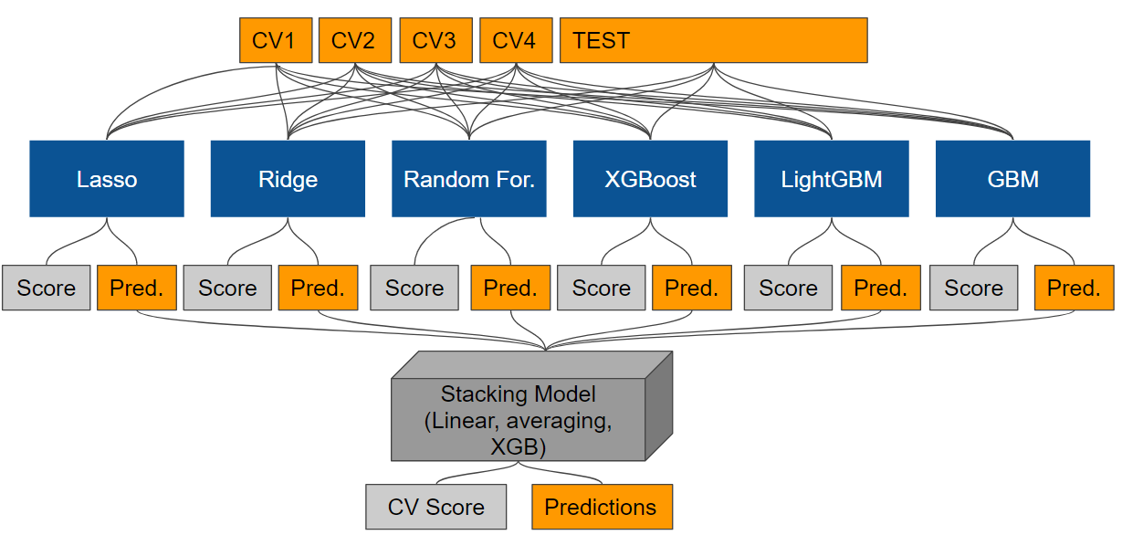
Essentially when one runs housing_main.py, it creates and trains a specified list of models in a sequence. For each model, it builds the model, fits the model with KFold cross validation (CV) with the training set, computes CV score, and also creates predictions on the Kaggle test set. The predictions on the training set (through KFolds CV) and the predictions on the Kaggle test set are then sent through the stacking pipeline. The stacker (either XGB, linear, or averaging) is then used to combine the models predictions to again get CV score and again create new Kaggle test set predictions. The final Kaggle test set predictions are saved to a .csv file for later use. Below is a graphical representation of the modeling process.
One may notice that there is no accounting here for the out-of-bag error (OOB), or a completely separate validation set. The models and their parameters were chosen largely due to their CV scores, so this inherently leads to some data leakage during CV. Future work would be to set aside maybe 20-30% of the initial training dataset to serve as an untouched validation dataset.
4. The Results
Ultimately, our rmsle was .12186 (898/4396 on Kaggle Leaderboard), which equates to our prediction being approximately an average of 13% off the true home value. Interestingly, the test error was about .012 higher than the CV error. As was mentioned previously, this may have been due to slight model and parameter overfitting while training.
5. The Future
If we were to work more on this project we would do a number of things differently. First, we would implement a recursive feature engineering to feature importance cycle so as to help home in on good features and develop a more accurate model. This would be aided with functional based ways to find feature importance so as to accelerate the process.
Second, we would implement a better testing method. As has been mentioned, the CV error should not be the only error with which we can gauge our model. In fact, the CV error is meant as a tool to choose models, refine models (parameter tuning), and avoid overfitting among other uses. However, it does not serve as a replacement for a test set to give an accurate estimate of one's test error. Furthermore, one does not want to submit often to Kaggle, as this is the true test score and one should avoid frequent submissions as this will lead to overfitting. Therefore, to avoid this, one should use an out of bag error by setting aside part of our training set at the start (20% perhaps).
Finally, we would investigate more into the effects of time as there is clearly a trend in housing price from 2006 to 2010 in United States, so it is curious that the dataset does not seem to reflect this.
Thank you for reading!


