Data Analysis of NYC Restaurant Sanitation data using R
Project GitHub | LinkedIn: Niki Moritz Hao-Wei Matthew Oren
The skills we demoed here can be learned through taking Data Science with Machine Learning bootcamp with NYC Data Science Academy.
Contributed by Marifel Corpuz.Marifel took R003 class with Vivian Zhang (Data Science by R, Intensive beginner level) in Mar - Apr, 2014 and did great in class. The post was based on her final project.
Videos:
This project is to demonstrate how to use R and NYC restaurant sanitation open data to analyze growth in number of restaurants in New York City, their scores, grades and violations.
# Required packages

library(gdata)
library(plyr)
library(reshape2)
library(ggplot2)
library(RXKCD)
library(tm)
library(wordcloud)
library(RColorBrewer)
First step is to download and read the tables into R. The following data sources are zipped and can be downloaded from: https://data.cityofnewyork.us/Health/Restaurant-Inspection-Results/4vkw-7nck?
(1). WebExtract.txt , (2) Cuisine.txt , (3) Violation.txt
WEBEXTRACT_0 <- read.delim("WebExtract.txt", fill = TRUE, as.is = TRUE, col.names = "V1",
    flush = TRUE, allowEscapes = FALSE, encoding = "iconv file.pcl -f UTF-8 -t ISO-8859-1 -c",
    stringsAsFactors = FALSE, fileEncoding = "latin1", strip.white = TRUE)

CUISINE <- read.table("Cuisine.txt", sep = ",", header = TRUE)

VIOLATION <- read.delim("Violation.txt", fileEncoding = "Latin1")
VIOLATION_FINAL <- as.data.frame(cbind(
    substr(VIOLATION$STARTDATE.ENDDATE.CRITICALFLAG.VIOLATIONCODE.VIOLATIONDESC,
    1, 19), substr(VIOLATION$STARTDATE.ENDDATE.CRITICALFLAG.VIOLATIONCODE.VIOLATIONDESC,
    21, 39), substr(VIOLATION$STARTDATE.ENDDATE.CRITICALFLAG.VIOLATIONCODE.VIOLATIONDESC,
    41, 41), substr(VIOLATION$STARTDATE.ENDDATE.CRITICALFLAG.VIOLATIONCODE.VIOLATIONDESC,
    43, 45), substr(VIOLATION$STARTDATE.ENDDATE.CRITICALFLAG.VIOLATIONCODE.VIOLATIONDESC,
    45, 45), substr(VIOLATION$STARTDATE.ENDDATE.CRITICALFLAG.VIOLATIONCODE.VIOLATIONDESC,
    47, 650)), )
After importing the files, the following are necessary steps to prepare the data for various analyses.
# Split column V1 in WEBEXTRACT_0 and rename the columns accordingly

WEBEXTRACT_1 <- with(WEBEXTRACT_0, cbind(colsplit(V1, pattern = ",", names = c("CAMIS",
    "DBA", "BORO", "BUILDING", "STREET", "ZIPCODE", "PHONE", "CUISINECODE",
    "INSPDATE", "ACTION", "VIOLCODE", "SCORE", "CURRENTGRADE", "GRADEDATE",
    "RECORDDATE"))))

# Rename the columns in VIOLATION_FINAL accordingly

VIOLATION_FINAL <- as.data.frame(rename.vars(VIOLATION_FINAL, c("V1", "V2",
    "V3", "V4", "V5", "V6"), c("STARTDATE", "ENDDATE", "CRITICALFLAG", "VIOLCODE",
    "VIOLATION", "VIOLATIONDESC")))
VIOLATION_FINAL$STARTDATE <- as.Date(VIOLATION_FINAL$STARTDATE)
VIOLATION_FINAL$ENDDATE <- as.Date(VIOLATION_FINAL$ENDDATE)

# Remove records where values of GRADEDATE column in WEBEXTRACT_1 contain letter

WEBEXTRACT_1 <- subset(WEBEXTRACT_1, grepl("^/l", WEBEXTRACT_1$GRADEDATE) ==  FALSE)

# This step is to remove white spaces
WEBEXTRACT_1 <- as.data.frame(apply(WEBEXTRACT_1, 2, function(x) gsub("s+", " ", x)))
Now, we left join the CUISINE table to the main table WEBEXTRACT_1 using CUISINECODE and perform additional data clean up.
WEBEXTRACT_2 <- merge(WEBEXTRACT_1, CUISINE, by = "CUISINECODE", all.x = TRUE)

# Convert the column INSPDATE from WEBEXTRACT_2 into date.
WEBEXTRACT_2$INSPDATE <- as.Date(WEBEXTRACT_2$INSPDATE)

# Add a new column INSPYEAR which is an extract from the column INSPDATE
WEBEXTRACT_2$INSPYEAR <- substr(WEBEXTRACT_2$INSPDATE, 1, 4)

# Last part of the data clean up is to recode the values of BORO into their proper names

WEBEXTRACT_2$BORO <- mapvalues(WEBEXTRACT_2$BORO, c("1", "2", "3", "4", "5"),
    c("MANHATTAN", "THE BRONX", "BROOKLYN", "QUEENS", "STATEN ISLAND"), warn_missing = TRUE)
In our analysis, we only want to focus on inspection years 2011 - 2013. We also want to make sure that each restaurant identified by a unique ID CAMIS has an assigned Borough (BORO) and cuisine type (CODEDESC).
The following steps are to prepare the data having the count of restaurants by Borough.
WEBEXTRACT_from2011 <- subset(WEBEXTRACT_2, WEBEXTRACT_2$INSPYEAR == c("2011",
    "2012", "2013") & WEBEXTRACT_2$BORO != "0" & is.na(WEBEXTRACT_2$CODEDESC) != TRUE)

# GET ALL UNIQUE COMBINATIONS OF CAMIS, INSPYEAR AND BORO
COUNT_byYEAR_byBORO <- unique(WEBEXTRACT_from2011[, c("CAMIS", "INSPYEAR", "BORO")])
COUNT_byYEAR_byBORO <- count(COUNT_byYEAR_byBORO, c("INSPYEAR", "BORO"))
Plot the count of restaurants by year and by Borough.
ggplot(COUNT_byYEAR_byBORO, aes(x = INSPYEAR, y = freq, fill = BORO)) + geom_bar(stat = "identity",
    position = "stack") + geom_text(data = COUNT_byYEAR_byBORO, aes(label = freq),
    size = 5, hjust = 0.5, vjust = 2, position = "stack") + xlab("Inspection Year") +
    ylab("Count of Restaurants") + labs(title = "Count of Restaurants in 2011-2013 in the 5 NYC BOROUGHs") +
    guides(fill = guide_legend(title = "NYC BOROUGHs"))
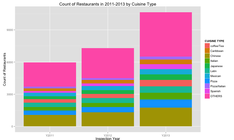
The following steps are to prepare the data having the count of restaurants by Cuisine Type. This is to show the growth by type of restaurants in NYC.
### GET ALL UNIQUE COMBINATIONS OF CAMIS, CODEDESC (CODE FOR CUISINE TYPE), INSPYEAR AND BORO
COUNT_CUISINE_byYEAR <- unique(WEBEXTRACT_from2011[, c("CAMIS", "CODEDESC",  "INSPYEAR", "BORO")])

### COUNT THE NUMBER OF CAMIS (UNIQUE IDENTIFIER OF RESTAURANT) BY INSPYEAR AND CODEDESC (CODE FOR CUISINE TYPE)
COUNT_CUISINE_byYEAR <- count(COUNT_CUISINE_byYEAR, c("CODEDESC", "INSPYEAR"))

### USE DECAST FUNCTION TO CREATE A HORIZONTAL FORMAT OF THE TABLE

COUNT_CUISINE_byYEAR_dcast <- dcast(COUNT_CUISINE_byYEAR, CODEDESC ~ paste0("Y", INSPYEAR), value.var = "freq")

### SORT THE TABLE IN DESCENDING ORDER OF NUMBER OF RESTAURANTS IN 2013 BY CODEDESC OR CUISINE TYPE
COUNT_CUISINE_byYEAR_SRTD <- COUNT_CUISINE_byYEAR_dcast[order(-COUNT_CUISINE_byYEAR_dcast$Y2013), ]


### GET THE TOP 10 MOST NUMBER OF CODEDESC OR CUISINE TYPE IN 2013
top10freq_2013 <- head(COUNT_CUISINE_byYEAR_SRTD, 10)

### ISOLATE THE RESTAURANTS THAT DON'T BELONG TO THE TOP 10 AND GROUP THEM AS 'OTHERS'
below10freq <- COUNT_CUISINE_byYEAR_SRTD[(COUNT_CUISINE_byYEAR_SRTD$Y2013 < min(top10freq_2013$Y2013)), ]
below10freq <- colwise(.fun = sum, .cols = is.numeric, na.rm = TRUE)(below10freq)
below10freq$CODEDESC <- "OTHERS"

### USE rbind FUNCTION TO combine the top 10 and the below 10 data
COUNT_CUISINE_byYEAR <- rbind(top10freq_2013, below10freq)

### SHORTEN LONG VALUES OF CODEDESC OR CUISINE TYPE FOR BETTER GRAPHING
COUNT_CUISINE_byYEAR$CODEDESC <- mapvalues(COUNT_CUISINE_byYEAR$CODEDESC, c("Cafxe9/Coffee/Tea",
    "Latin (Cuban, Dominican, Puerto Rican, South & Central American)"), c("coffee/Tea",
    "Latin"), warn_missing = TRUE)

### USE THE melt FUNCTION TO REFORMAT THE TABLE INTO A LONG FORM FOR PLOTTING
COUNT_CUISINE_byYEAR <- melt(data = COUNT_CUISINE_byYEAR, id.vars = c("CODEDESC"))
Plot the count of restaurants by Cuisine Type.
ggplot(COUNT_CUISINE_byYEAR, aes(x = variable, y = value, fill = CODEDESC)) +
    geom_bar(stat = "identity", position = "stack") + xlab("Inspection Year") +
    ylab("Count of Restaurants") +
    labs(title = "Count of Restaurants in 2011-2013 by Cuisine Type") +
    guides(fill = guide_legend(title = "CUISINE TYPE"))
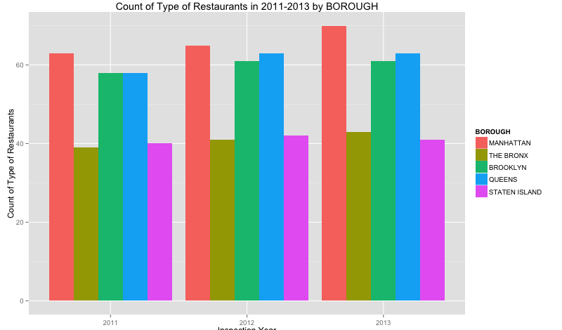
The following steps are to prepare the data having the count of cuisine types by Borough. This is to show what type of restaurants are more prevalent in each borough and which one is increasing in number in 2011-2013.
### GET ALL UNIQUE COMBINATIONS OF CODEDESC (CODE FOR CUISINE TYPE), INSPYEAR AND BORO
UNIQ_CUISINE_byYEAR_byBORO <- unique(WEBEXTRACT_from2011[, c("CODEDESC", "INSPYEAR", "BORO")])

### COUNT THE NUMBER OF CAMIS (UNIQUE IDENTIFIER OF RESTAURANT) BY INSPYEAR AND CODEDESC (CODE FOR CUISINE TYPE)
UNIQ_CUISINE_byYEAR_byBORO <- count(UNIQ_CUISINE_byYEAR_byBORO, c("BORO", "INSPYEAR"))
Plot the count of Cuisine Type by Borough.
ggplot(UNIQ_CUISINE_byYEAR_byBORO, aes(x = INSPYEAR, y = freq, fill = BORO)) +
    geom_bar(stat = "identity", position = "dodge") + xlab("Inspection Year") +
    ylab("Count of Type of Restaurants") +
    labs(title = "Count of Type of Restaurants in 2011-2013 by BOROUGH") +
    guides(fill = guide_legend(title = "BOROUGH"))
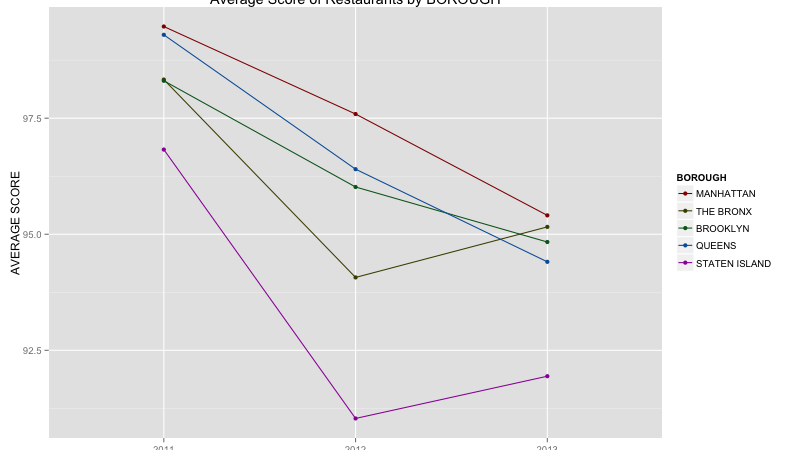
The following steps are to analyze the sccores of Restaurants that were inspected in 2011, 2012 and 2013.
## USING THE aggregate FUNCTION, CALCULATE THE AVERAGE SCORE OF EACH BOROUGH BY YEAR,
BUT CONVERT THE SCORE COLUMN FIRST INTO A SCORE

WEBEXTRACT_from2011$SCORE <- as.numeric(WEBEXTRACT_from2011$SCORE)
AGG_SCORE <- aggregate(WEBEXTRACT_from2011$SCORE, by = list(WEBEXTRACT_from2011$BORO,
    WEBEXTRACT_from2011$INSPYEAR), FUN = mean, na.rm = TRUE)
Plot the average scores of restaurants by Borough.
ggplot(AGG_SCORE, aes(Group.2, x, group = Group.1, colour = Group.1)) + geom_line() +
    geom_point() + scale_colour_hue(name = "BOROUGH", l = 30) + xlab("Inspection Year") +
    ylab("AVERAGE SCORE") + labs(title = "Average Score of Restaurants by BOROUGH") +
    guides(fill = guide_legend(title = "BOROUGH"))
Here, we want to show the distribution of grades of restaurants by Borough.
### GET ALL UNIQUE COMBINATIONS OF CAMIS(CODE FOR RESTAURANT), CODEDESC (CODE FOR CUISINE TYPE),
INSPYEAR AND BORO
COUNT_GRADE_byYEAR <- unique(WEBEXTRACT_from2011[, c("CAMIS", "INSPYEAR", "CURRENTGRADE", "CODEDESC", "BORO")])

### GROUP BY CURRENTGRADE, INSPYEAR AND BORO
COUNT_GRADE_byYEAR <- count(COUNT_GRADE_byYEAR, c("CURRENTGRADE", "INSPYEAR",  "BORO"))

### CONVERT THE CURRENTGRADE FIELD TO CHARACTER

COUNT_GRADE_byYEAR$CURRENTGRADE <- as.character(COUNT_GRADE_byYEAR$CURRENTGRADE)

### REMOVE RECORDS WHERE CURRENTGRADE IS NOT A,B,C,P OR Z FOR INSPYEAR = 2013

COUNT_GRADE_byYEAR <- subset(COUNT_GRADE_byYEAR, (COUNT_GRADE_byYEAR$INSPYEAR ==  "2013") &
                       (COUNT_GRADE_byYEAR$CURRENTGRADE %in% c("A", "B", "C", "P", "Z")))
Plot the count of Restaurants by Grade by Borough.
ggplot(COUNT_GRADE_byYEAR, aes(x = BORO, y = freq, fill = CURRENTGRADE)) + geom_bar(stat = "identity",
    position = "stack") + xlab("NYC BOROUGHs") + ylab("Count of Restaurants") +
    labs(title = "Count of Restaurants inspected and Graded in 2013") +
    guides(fill = guide_legend(title = "GRADE"))
Lastly, we want to illustrate the different violations in all restaurants inspected in 2013. We also want to compare this to the violations incurred by restaurants that were graded A in 2013.
#### GET THE LATEST INSPECTION DATES FOR ALL INSPECTION APPLICABLE IN 2013
LATEST_INSPECTIODATE <- max(VIOLATION_FINAL$STARTDATE)

#### SUBSET FROM VIOLATION TABLE LATEST LIST OF RESTAURANT VIOLATIONS
RECENT_VIOL_REF <- subset(VIOLATION_FINAL, (VIOLATION_FINAL$STARTDATE == LATEST_INSPECTIODATE))


### GET ALL UNIQUE COMBINATIONS OF CAMIS(CODE FOR RESTAURANT), CODEDESC (CODE FOR CUISINE TYPE), INSPYEAR
AND BORO AND CURRENTGRADE
VIOLATION_DATA_WORDMAP <- unique(WEBEXTRACT_from2011[, c("CAMIS", "INSPYEAR",
    "VIOLCODE", "CODEDESC", "BORO", "CURRENTGRADE")])

### MERGE TO VIOLATION DATA ON VIOLCODE TO GET DESCRIPTIONS OF VIOLATIONS
VIOLATION_DATA_WORDMAP <- merge(VIOLATION_DATA_WORDMAP, RECENT_VIOL_REF, by = "VIOLCODE", all.x = TRUE)
Create a word cloud to illustrate the frequency of violations in restaurants inspected in 2013.
# WordCloud related to violations of all NYC restaurants inspected in 2013

xkcd.corpus <- Corpus(DataframeSource(data.frame(VIOLATION_DATA_WORDMAP[, "VIOLATIONDESC"])))
xkcd.corpus <- tm_map(xkcd.corpus, removePunctuation)
xkcd.corpus <- tm_map(xkcd.corpus, tolower)
xkcd.corpus <- tm_map(xkcd.corpus, function(x) removeWords(x, stopwords("english")))
xkcd.corpus <- tm_map(xkcd.corpus, function(x) removeWords(x, c("andor", "food", "foods", "properly", "improperly", "maintained", "provided")))
myDTM = TermDocumentMatrix(xkcd.corpus, control = list(minWordLength = 1))
m <- as.matrix(myDTM)
v <- sort(rowSums(m), decreasing = TRUE)
d <- data.frame(word = names(v), freq = v)
pal <- brewer.pal(9, "Spectral")
pal <- pal[-(1:2)]
wordcloud(d$word, d$freq, scale = c(8, 0.3), min.freq = 5, max.words = Inf, random.order = F, rot.per = 0.15, colors = pal, vfont = c("sans serif", "plain"))
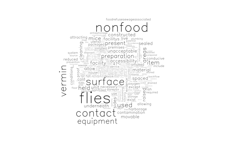 Subset the data to have only the Grade A restaurants then create a word cloud of the violations.
VIOLATION_DATA_WORDMAP_A <- subset(VIOLATION_DATA_WORDMAP, CURRENTGRADE == "A")
# WordCloud related to violations of all Grade A NYC restaurants inspected in 2013

xkcd.corpus <- Corpus(DataframeSource(data.frame(VIOLATION_DATA_WORDMAP_A[,
    "VIOLATIONDESC"])))
xkcd.corpus <- tm_map(xkcd.corpus, removePunctuation)
xkcd.corpus <- tm_map(xkcd.corpus, tolower)

xkcd.corpus <- tm_map(xkcd.corpus, function(x) removeWords(x, stopwords("english")))
xkcd.corpus <- tm_map(xkcd.corpus, function(x) removeWords(x, c("andor", "food",
    "foods", "properly", "improperly", "maintained", "provided")))
myDTM = TermDocumentMatrix(xkcd.corpus, control = list(minWordLength = 1))

m <- as.matrix(myDTM)
v <- sort(rowSums(m), decreasing = TRUE)
d <- data.frame(word = names(v), freq = v)
pal <- brewer.pal(9, "Spectral")
pal <- pal[-(1:2)]
wordcloud(d$word, d$freq, scale = c(8, 0.3), min.freq = 5, max.words = Inf,
    random.order = F, rot.per = 0.15, colors = pal, vfont = c("sans serif",
        "plain"))


