Examining Billboard Hot 100 Lyrics from 1987 - 2016

Going back to August 4th, 1958, Billboard has released a weekly publication of the "Hot 100" Singles chart
Introduction - Billboard magazine cemented their status as an integral figure of American popular culture with the creation of the Billboard Hot 100 chart. Since 1958, the Hot 100 chart has been accepted as the 'gold standard,' or benchmark of the popular music rankings.
The rankings are based on a formulaic approach, not the subjective to the musical preferences of the individuals tasked with compiling the list. Airplay on roughly one thousand terrestrial radio stations are tracked to form the foundation of the ranking data. Nielsen provides song sales data for both digital and physical formats which are factored into the rankings. Most recently, Billboard added music streaming data to be factored into the hot 100 chart rankings.
Scope - For this project I wanted to analyze the lyrics from popular songs over the past 30 years. In order to have a consistent input source and not have my musical preferences bias the results of the analysis I chose to work with the Billboard Hot 100 charts. Billboard releases weekly Hot 100 charts going back to the 1950's. Click here to find This Week's Hot 100 Chart.
My goal was to analyze the lyrics by year, and find trends in the most popular words used .
Data - All data used in this project was scraped.
The Billboard Hot 100 chart data was scraped from The Ultimate Music Database using a combination of BeautifulSoup, and Regular Expressions.
The twsift unofficial API for MetroLyrics was used to acquire the lyrics corresponding to each song entry in the Billboard Hot 100 charts. This API allows quick access to the lyrical content hosted by MetroLyrics with one major caveat - the song title and artist must be meticulously adjusted (removing non alpha-numerical characters, replacing spaces with '-', and correctly identifying the title & artist) otherwise it wont return the correct lyrics.
Click here for lyric scraping code
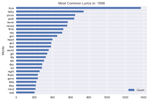
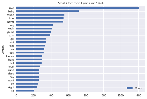
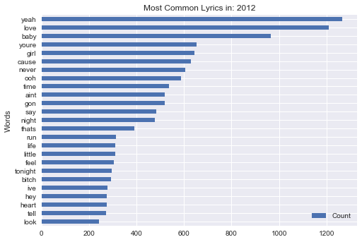
Top 25 Words per Year, 1988-2016
1988

1989
1990
1991
1992
1993
1994
1995
1996


2001
2002
2003
2004
2005
2006
2007
2008
2009
2010
2011
2012
2013
2014
2015
2016
Wordcloud by year from 1987-2016
1987

1988
1989

1990
1991
1992
1993
1994
1995
1996
1997
1998
1999

2000

2001

2002


2004
2005
2006

2007
2008
2009
2010
2011
2012
2013

2014
2015
2016
######Generate Word-cloud by year
from os import path
from wordcloud import WordCloud
def get_wordcloud_year(year):
wordbag = words_by_year(year)
words = remove_nonalphanum(wordbag)
print 0, len(words)
words = words.split()
# Remove single-character & 2-character tokens (mostly punctuation)
words = [word for word in words if len(word) > 2]
print 1, len(words)
# Remove numbers
words = [word for word in words if not word.isdigit()]
print 2, len(words)
# Lowercase all words (default_stopwords are lowercase too)
words = [word.lower() for word in words]
print 3, len(words)
#remove stopwords
words = [word for word in words if word not in all_stopwords]
print 4, len(words)
#wordcloud = WordCloud().generate(words)
# Display the generated image:
# the matplotlib way:
import matplotlib.pyplot as plt
# plt.imshow(wordcloud)
plt.axis("off")
# lower max_font_size
#wordcloud = WordCloud(max_font_size=50).generate() (str(words))
plt.figure()
#plt.imshow(wordcloud)
plt.axis("off")
#plt.show()
print(len(words))
wordcloud = WordCloud(width = 1000, height = 750, font_path='/Library/Fonts/Verdana.ttf',
relative_scaling = 1.0,
stopwords = all_stopwords,
).generate(' '.join(words))
plt.figure(figsize=(20,12))
plt.imshow(wordcloud)
plt.axis("off")
plt.show()
###Generates histogram of top 25 lyrics
stopwords_file = './stopwords.txt'
custom_stopwords = set(codecs.open(stopwords_file, 'r', 'utf-8').read().splitlines())
all_stopwords = default_stopwords | custom_stopwords
def get_wordfreq_df(year):
wordbag = words_by_year(year).decode('utf-8')#vocab.decode('utf-8')#words_by_year(year)
words = nltk.word_tokenize(wordbag)
words = [word for word in words if len(word) > 2]
words = [word for word in words if not word.isdigit()]
words = [word.lower() for word in words]
words = [word for word in words if word not in all_stopwords]
fdist = nltk.FreqDist(words)
d = Counter(fdist)
word_df = pd.DataFrame.from_dict(d, orient='index').reset_index()
word_df = word_df.rename(columns={'index':'Word',0:'count'})
df = pd.DataFrame(fdist.most_common(25))
df.columns = ['Words', 'Count']
df.sort_index(ascending=False).plot(
kind='barh',
x = 'Words',
title = "Most Common Lyrics in: " + year,
)
Conclusion - A lot has changed in regards to popular music over the past 30 years, but one theme stands the test of time - Love. Although in recent years its lead seems to be fading (though that may be an artifact of my data collection), "Love" is consistently one of the most frequently used words in popular music
The most frequent words in the Billboard Hot 100 lyrics since 1987 are:
I'm
Love
Don't
Like
Know
Oh
Just
Got
Baby
Yeah
Want
You're
Cause
Make
Time
Let
Girl
Say
Way
Come
I'll
Ain't
Right
Gonna
Need