Customer Lifetime Value Product Recommendation for Retail
Project GitHub | LinkedIn: Niki Moritz Hao-Wei Matthew Oren
The skills we demoed here can be learned through taking Data Science with Machine Learning bootcamp with NYC Data Science Academy.
Introduction
On any given day, countless transactions are being made in the retail space. All the transactions generate data, which can be utilized by merchants to improve their sales and help them make important business decisions. As part of our capstone, we consulted two retail clients to explore and identify trends in their customer behavior by building visualizations as well as predictive models. We have split the blog into 2 parts to represent our exploration and modeling for the respective clients and dataset.
Part 1. Predictive Customer Lifetime Value and Product Recommendation for Retail
1.Exploratory Data Analysis (EDA)
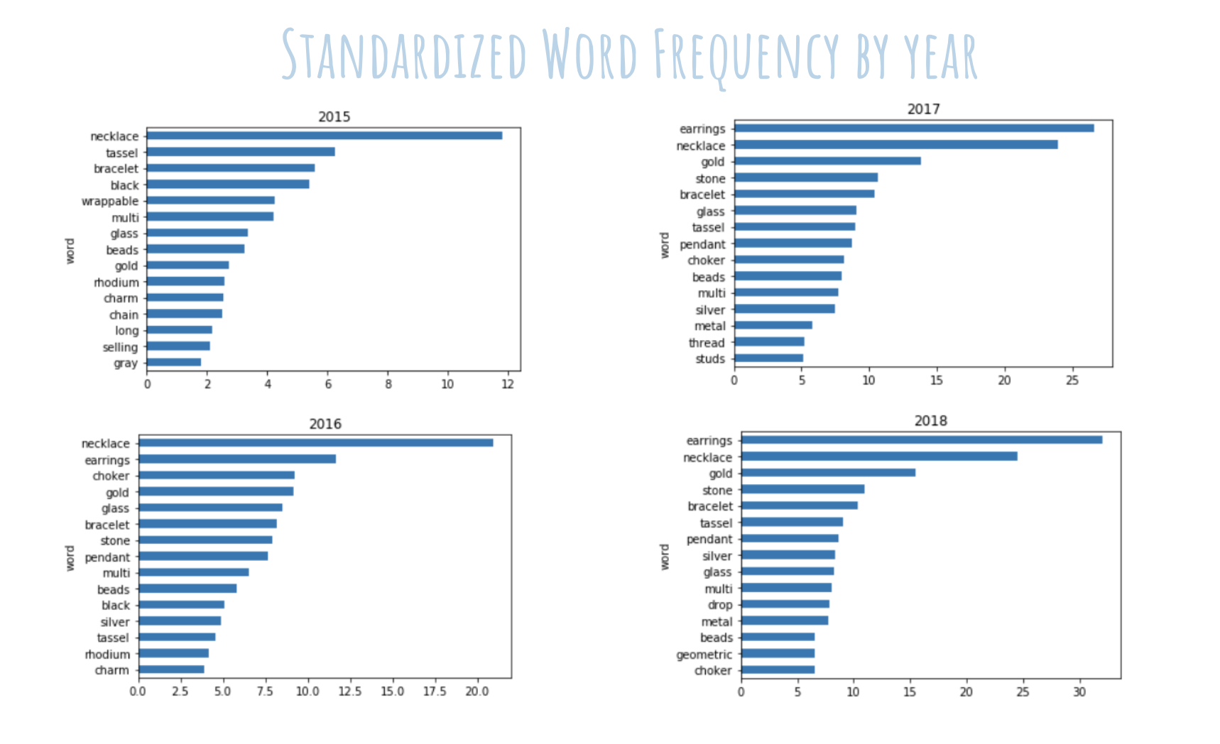
Upon receiving the data for the first client, we realized that the product items listed were in a semi-structured format. That is, some of the item names were in a “product name – color” format, although there were many items that did not have that format. That made it difficult to separate out the product with the color. To simplify things, we decomposed all the item names into individual words in a corporus, thereby allowing us to see the top generic items/color sold by analyzing the word count frequency.
We wanted to analyze any sales and item trends by year, so the frequency was standardized to show a meaningful comparison across years. As the graphs below show: necklaces/earrings are hot sellers. And gold colored jewelry are in demand.
For retailers, November tends to be the month of high sales volume due to the holiday season and Black Friday deals. We wanted to see if there were any specific trends in November that can allow the business to determine when is the best time to increase their advertising budget and promotional efforts. Indeed, we recognized that the first week of November in every year has the weakest sales volume. Therefore, we advised the company to perhaps spend more marketing dollars on the first week as an early holiday special promotion.
2. Modeling
2.1 RFM Segmentation, Analysis and Model
Since we did not have a target variable to predict, we had to get creative during our modeling phase. After doing some research, we decided to first do an RFM analysis (recency, frequency, monetary). The goal of RFM analysis is to utilize data regarding the recency (how recently a customer has purchased), frequency (the number of repeat purchases of a customer), and the monetary value of the orders to determine how valuable a customer is, as well as how many times a customer will return over the course of the next x time periods.
In our case, we were specifically interested in the CLV (customer lifetime value) and the number of times a customer will return. We used these results to perform a customer segmentation by creating the additional variable “Target_Group.” Let’s begin with data preparation.
In order to perform RFM analysis on our data, we had to transform it. Luckily, the “lifetimes” package in Python provides a function to do so. After having transformed our data, our data frame looked like this:
The ‘T’ column in this data frame simply represents the age of each customer. Equipped with our prepared data, we first investigated the specific characteristics of our clients’ best customers with regards to frequency and recency. We decided to plot our result using a heatmap that turns more yellow if a customer is more likely to return within the next period of time (as part of the data preparation, you have to specify a unit of time you want to base your analysis on; we set this parameter to ‘M’ for months).
This heatmap shows that the customers most likely to return have a historical frequency of around 16, meaning they’ve came back to purchase again 16 times, and a recency a little over 30, meaning that these customers had an age of a little over 30 when they last purchased.
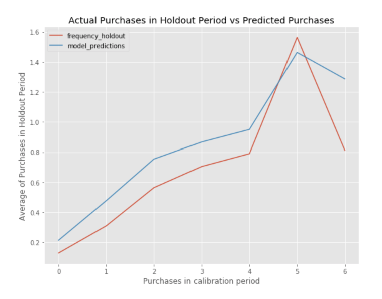
Before starting to segment our clients’ customers, we wanted to make sure the model we were using was making accurate predictions. As in other machine learning approaches to prevent overfitting, we divided our data in a calibration and holdout set. Then, we fit the model on our calibration set and made predictions on the holdout set that the model had not seen yet.
Since we only had data for a relatively short period of time, we used the last 6 months of our data to test our model and got the below result. As we can see, despite our model not fitting the actual purchases perfectly, it was able to capture trends and significant turning points over the course of six months:
While this information is valuable, it does not satisfy our goal for insights yet. We wanted to produce actionable insights that could be implemented immediately to create business value. To do so, we decided to take a look at the number of times a customer is predicted to return within the next month, which can be interpreted as the probability of the customer returning in the next month.
Based on these insights, customers most likely to return can be targeted specifically with ad/marketing campaigns. By doing so, the amount of money spent on marketing can be reduced, and the return on these expenses can be increased.
We also included a more generalized version of this technique in our final product that, after specifying a time range and selecting a customer, returned the number of expected repeat purchases by this specific customer.
The other aspect of RFM analysis that we were really interested in as a basis for our clustering was the CLV. Calculating the CLV using the “lifetimes” package is really easy once you’ve prepared your data the right way. In order to be able to use the DCF (discounted cash flow) method, we needed to add a column with the monetary .
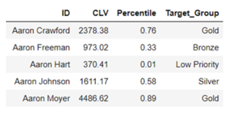
Then, it was just a matter of fitting the model and making the computation. We then sorted our data in an descending order to identify the most valuable customers for our clients. Here is an example of what our result looked like: We also wanted to let our clients know the probability of a particular customer to make returning purchases.
In other words, we needed to understand the probability that the customer is still “alive” or active in the customer lifecycle. The “lifetimes” Python library includes the tools to allow us to do these types of analyses. Take for instance the following customer, who made their initial purchase back in October of 2016 and hasn’t made another purchase for a few months. The likelihood of the customer being a recurring customer drops until they make their second purchase.
For the client, this information can be used to signal when to send out customer targeted promotions whenever the customer aliveness probability drops below a certain threshold. In the life cycle plot below, the dashed lines represent a purchase and the normal line describe the probability of this customer being alive at that specific date.
From a business perspective, it may also be helpful to segment customers based on their buying patterns. There are many ways to do this; the route we took was to use the CLV , mapping them to their corresponding percentiles and finally binning them to “Low Priority, Bronze, Silver, Gold”. Through this approach, Company A can easily see who are their most important customers and also create new strategies to bump lower tier customers to the higher tiers.
One such approach that we recommended was to have tier specific rewards program and to include periodic progress email to the customer to let them know how close they are to reaching the next tier in an attempt to encourage higher purchasing volume.
2.2 Association Rules and the Apriori Algorithm
Another model we utilized was the product recommendation system that pushes potentially interesting products to customers. One of the bigger costs in the retail business is the cost of unsold inventory that sits in the warehouse. To solve this problem, we designed a recommendation system utilizing associated rules with an added feature. The system allows the business to input items that they want to move from their inventory, and the recommendation system will prioritize those items if it is associated with items that a customer has or intends to purchase.
The system was based on a priori, or associated learning algorithm. It is an algorithm for frequent itemset mining over transactional database. The goal is to find high frequent item combination in transactions and make “rules” to make decisions to recommend products.
Each rule has three parameters: support, confidence, and lift. Generally speaking, it is desirable to use the rules with high support. These rules will be applicable to a large number of transactions and are more interesting and profitable to evaluate from a business standpoint.
The biggest challenge we encounter in rule mining was due to the unique nature of the client’s customers. As the customers are businesses and not normal retail customers, the rules that were generated were not unique. For example, jewelry retailers will buy earrings across multiple colors in bulk to appeal to different customers, whereas an individual retail customer will purchase just one or 2 colors for any particular item.
The result is that a rule generated will be that customers who buy “Gold Earring” will also buy “Silver Earring,” which is not insightful (we want to generate rules between different products).
To achieve the goal of generating more meaningful rules, we created a new feature which is “vendor : category”. As its literal meaning, this feature stores the vendor and category information of each item. By using this feature instead of line item in transaction, we were able to decrease the computation burden and also resolve the problems discussed above, thereby acquiring interesting rules.
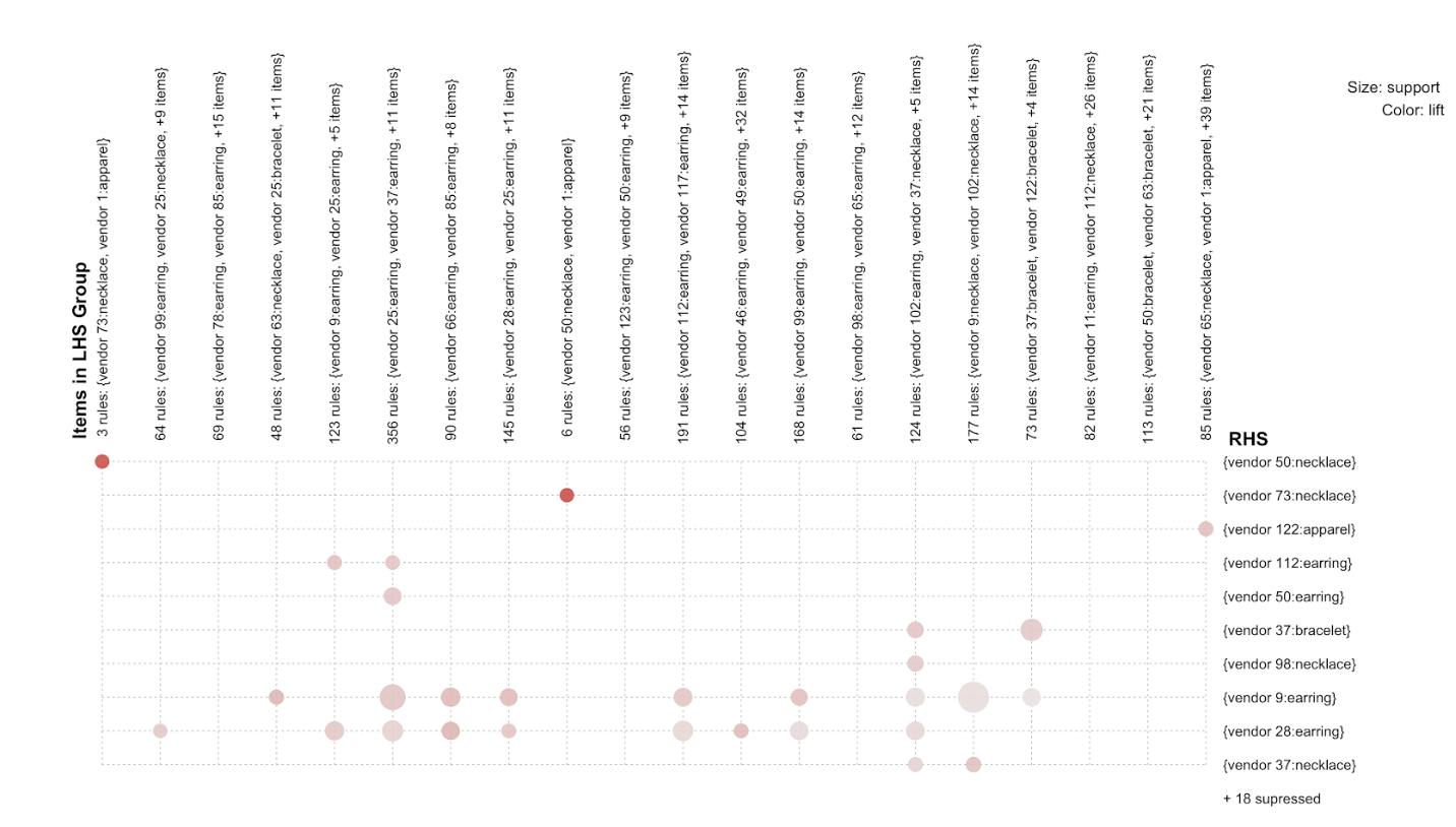
The following figure is an example of the new rules created using the R package “arules”. Comparing to its peer python packages, it shows more completed result. R provides robust visualization tools for a priori, “arulesViz,” which is not compatible in Python. The figure below shows a sample of three rules of total 2138 rule. For rule arrows pointing from item to rule vertices indicate LHS items and from rule to item represent RHS. The size of rules vertices indicates support of the rules, and color indicates lift. Larger size and darker color mean higher support and lift, respectively.
Graph-based plot with items and rules as vertices (3 rules)
Grouped Matrix-based plot (2138 rules)
The next step is to push products based on the rules. Here is how our model works: first, once customer generate an order, each item in the order will be transformed into “vendor : category” type, and create LHS “vendor : category” list; second, the model will look up rules library, and generate the highest support RHS “vendor : category” list according to the LHS; third, find all items under RHS “vendor : category” list, and rank them by their frequency, then recommend the top three frequency items.
As mentioned at the beginning of this section, our model has a unique feature of enabling businesses to direct attention to items they want to offload. This is done by modifying the third step. Let’s say, the business created a list of items which make up a lot of inventory in the warehouse, if these items happen to appear in the items under RHS “vendor : category” list, they will override the whole rank and are pushed to customers.
Conclusion
Through the CLV analysis and improved recommendation system, we aimed to help the business better target customer segmentation and help with their inventory turnover ratio. We’ve learned a great deal in working with this business in that applying our data science skill sets to a real world environment is often quite different than the classroom setting. In part 2, we will continue our journey with yet another retail company and hope to uncover hidden sales patterns through a Shiny dashboard as well as forecast future sales from a time series analysis.


