Data Object Localization using Bounding Boxes Deep Learning
Project GitHub | LinkedIn: Niki Moritz Hao-Wei Matthew Oren
The skills we demoed here can be learned through taking Data Science with Machine Learning bootcamp with NYC Data Science Academy.
An Image Processing Project based on Neural Network Deep Learning
Sponsored by Koios Medical, this project aims to build a deep learning neural network model that can localize potential tumors and/or lesions on ultrasound scans of the thyroid. This model is trained on a data set of patient thyroid scans that have already been marked by radiologists, available here (based on this research paper). The model is built on the Keras framework (using tensor flow on the backend) and utilizes the Xception pre-trained weights to initialize its training.
The code for this project can be found here.
Project Background
This capstone project for the NYC Data Science Academy was sponsored by Koios Medical. The project was aimed at developing a reliable model that can essentially automate the particular function of the radiologist, whereby they mark/ identify potential lesions or tumors for further biopsy or investigation. The envisioned benefit of using a machine learning method is that it can possibly identify areas of interest that might be missed by a human radiologist due to image quality, error or any other reason, while also increasing efficiency in reporting test results to physicians. The model itself, however, was designed to train for this task using marks already made by radiologists from the publicly available data set linked above.
Project Data and Image Augmentation
The data in this project consists of black and white images ( grayscale with three "color-channels") of thyroid ultrasound scans, that were sized either (315 x 560) or (360 x 560) pixels. There were also .csv files that assigned image IDs to each scan and the corresponding directory path, as well as bounding box coordinates (upper left-hand side x and y values and the weight and height) alongside pixel values/ positions for segmentation purposes (alternate method of object localization).
There are 466 raw images from the dataset that were eventually used in this project, which is a rather scare quantity. Therefore, the first step was to augment these images to generate new data for modeling. The "imgaug" open source Python library was used to generate them. The following code snippet outlines the transformation parameters that were applied to the images:

Set of Image augmentation parameters. Relevant Imgaug documentation
To elaborate, 50% of the image set was randomly chosen to be horizontally flipped/ mirrored into new images. Additionally, the image contrast was varied randomly between 75% and 150% of the original contrast,, as well as brightness (between 80% and 120%) and finally, the rotation transformation between (-15 and 15 degrees).
Some of the scans in the dataset were "double" images, an example of which can be found below:
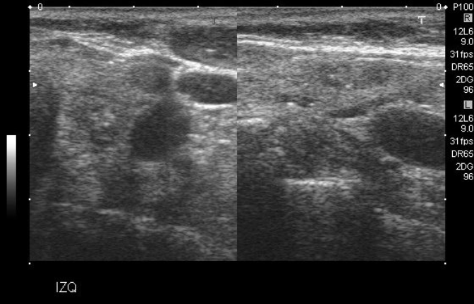
Example of a "double" image scan
Some of the limitations of the structure of this project and the model used meant that only one bounding box can be predicted per image. It is most definitely a severe limitation of this project which will be discussed later. However, at this point in the augmentation process, to maintain simplicity in the dataset, these "double" images were removed. There were 172 of them, thus reducing the 466 image set to 294.
The imgaug library allows the user to determine the number of new images to be augmented based on a multiplied factor of the original set of images. The final, augmented data set therefore included 3,234 images (294 original and 294 x 10 = 2,940 augmented). This was split into 60-20-20 training, validation and testing sets (3,175, 1,058 and 1,059 images respectively)
A sample augmentation is displayed below (the original and transformed image):
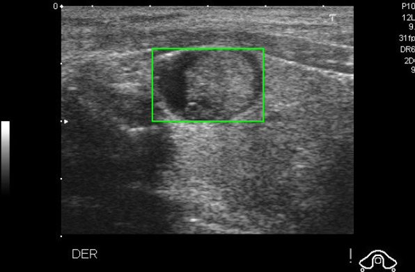
Pre-Marked Bounding Box on Ultrasound Scan
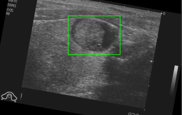
Translated Bounding Box on Augmented image (with transformations applied to the same prior image)
Project Model Architecture
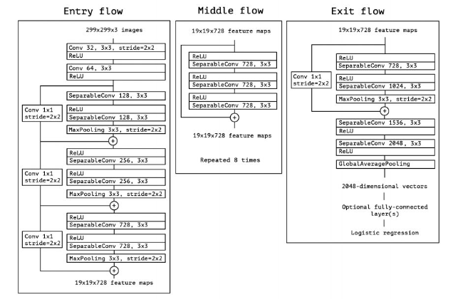
The neural network for this project was compiled, trained and tested using the Keras framework (using TensorFlow in the backend), as mentioned above. In fact, the Xception model was used to build this prediction model, including loading the pre-trained weights from ImageNet. Details can be found here. The following image is an outline of the layers that comprise of Xception. Clicking the image will lead to a concise explanation of this model.
While these models are typically used for object detection using a classification-problem approach, since our goal was simplified to consider only object localization prior to classification, as an exercise in learning and experimentation, the Xception model was modified to take on a regression-problem approach. In this case, the network seeks to "regress" the bounding box coordinates onto the images and predict them based on fitting to the pre-defined target variable (the set of coordinates in the dataset).
For the purposes of this project, once Xception was loaded on as the base layers (with an input image size of 299 x 299 x 3):
- A Flatten layer was added to begin extracting the bounding box coordinates after the images were analyzed and "seen" by the model.
- This was followed by a 50% Dropout layer to ease the computational burden from this model.
- Finally, two Dense layers were added to reduce the output dimensions down to 64, then finally 4 to correspond to the four points of the bounding box coordinates (technically two points: upper-left and lower-right corners). The Dense layers utilized a linear activation function.
The following is a code output of the model summary:
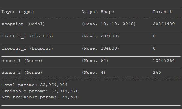
Model layers implemented (for this project specifically) after pre-trained Xception architecture was already loaded
Since Keras was being used, it allowed the creation of training, validation and test data "generators" that Keras then uses for fitting, optimizing and predicting. The Keras image-data-generators were built based on the flow_from_dataframe method - instead of using a set directory for the predictor or "feature" images, a "directory" variable (column) in the data frame corresponds to each image and the rows indicate the bounding box coordinates.
Project Model Performance
The model isn't particularly efficient and computationally very heavy, both due to the structure and code, as well as the nature of the problem itself. Processing over 3,000 images means a regular, personal laptop is not sufficient. As such, the project required the use of GPUs which were available for public use through the Google Colab service.
The neural network was fitted on the training and validation image sets over 25 epochs, the results of which are available below. This model was evaluated on two metrics. The first is a mean-squared error (MSE) loss, and the second is the IoU (Intersection over Union). A thorough explanation of IoU can be found here. The IoU metric had to be manually created as a TensorFlow and Python function since it is not a built-in metric for Keras. The two sources that were combined and used to this purpose can be found here and here.
On the first graph, we can see that the training and validation IoU scores are closely matched and they converge to a stabilized score of roughly 80% before the 10th epoch. In the second graph, we see the MSE loss drop to values close to zero from the 2nd epoch onwards. These results seem suspicious.
The first issue is that the validation scores are actually better than the training scores. This is a strong indicator of overfitting, however, some brief research has shown that this is a known consequence of the use of a Dropout layer (since a dropout layer removes observations during training, but leaves data in place during validation).
The next issue is the tremendously low MSE loss, which might still indicate overfitting and a possible case of data leakage. However, the results of the test set predictions might be more indicative.
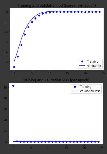
Training and Test set performances over 25 epochs. IoU scores (above) and MSE (mean-squared error) loss (below)
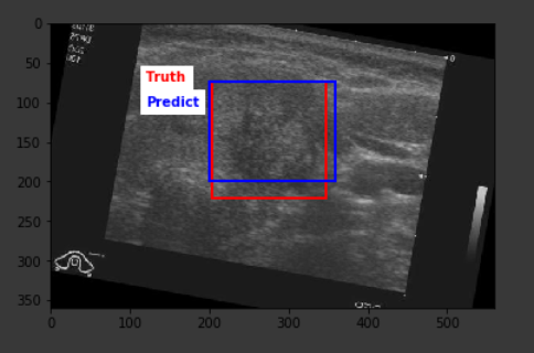
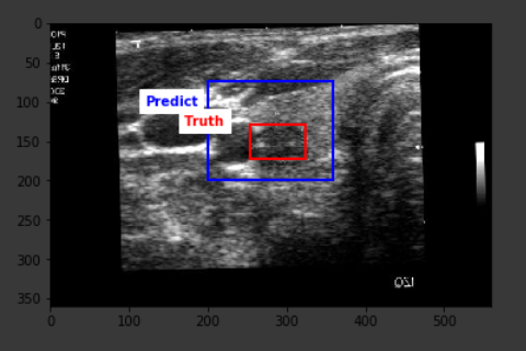
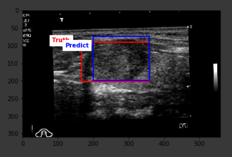
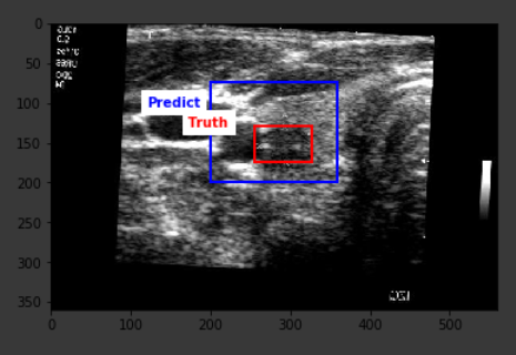
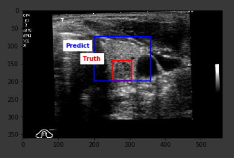
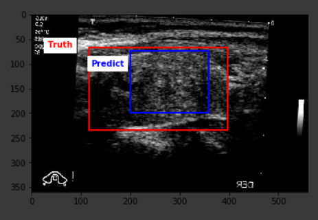
The average IoU score from the predictions on the test set turned out to be 42.3% with the highest score of 78.4%. The result is definitely far from optimal, but a closer look at the outcomes show that the predictions are definitely around the correct location on the image, however, the model falls short in being able to correctly predict the lesion size, hence the existing score.
Below are some sample outputs from the model prediction. The first image is the best IoU achieved. The rest are randomly chosen:
Project Conclusions and Future Work
There is definitely a lot of improvements to be made on this project and the model can certainly be tested with other parameters and changes. For example, the severe limitation of being able to predict only one set of bounding boxes per image, the resource-intensive structure of the project, the scarcity of data/ images, etc.
One of the changes that were considered was converting all the coordinate values from absolute values (pixels) to scaled values based on the image dimensions so that they would be bound between 0 and 1 in order to cater to TensorFlow's preference for small numbers. Additionally, a sigmoid activation function could be used on the dense layers instead of a linear one - as a test to see if it lead to better, more stabilized results.
However, as a first-time foray into deep learning and neural networks in general, this was a tremendous learning experience with tangible results. The goal is to continue learning and building on this progress and fine-tuning the techniques behind the project to achieve better and useful results.


