Data Visualization on Customer Experiences
The skills the author demoed here can be learned through taking Data Science with Machine Learning bootcamp with NYC Data Science Academy.
Contributed by Adam Owen. He is in the NYC Data Science Academy 12 week full time Data Science Bootcamp program taking place between January 11th to April 1st, 2016. This post is based on his fourth class project, Maching Learning (due on the 8th week of the program).
The Customer is Always Right. If you haven't heard that before, then you may have never worked in retail or attempted to return faulty Christmas toys on December 26th. Data shows angry consumers today not only leave forever but may also post nasty online reviews causing a ripple effect through the company's entire market. Santander, in its efforts to keep customers happy, deployed a Kaggle competition to predict customer satisfaction with $60,000 in prize money at stake. Needless to say, us Kagglers are keen to jump into the race.
DATA SET
The dataset provided includes ~70,000 train observations and ~70,000 test observations (does not include the dependent variable) of 370 anonymized continuous and categorical variables. Much like the real world, we don’t know exactly what’s going on with each variable and we will have to deploy our data scientist intuition and guile to detect feature significance.
To get a better understand the overall data structure, I’ve sampled 10% of the dataset and displayed it on the following heatmap.
It’s quickly apparent that ~91% of the dataset are zeros. Some of those zeros have meaning in categorical features and others may represent NAs. Also, there are several outlier variables that sit well above the mean such as all ‘delta*’ variables that have medians of ~2 and outliers around 100,000,000. Without the actual feature title to decipher precise meaning, we’ll have to explore a variety of feature engineering tricks.
FEATURE ENGINEERING
Correct feature engineering is the most difficult and rewarding task in most machine learning models. So, most of my time was spent in assessing various feature manipulations and testing the difference. After several feature adjustments, I’ve assembled base and advanced cases in feature engineering and later we’ll test the difference.
BASE CASE
The dependent variable is binary so we will explore a variety of logistic regression and decision tree models. The first feature selection will meet the assumptions of a logistic regression model including:
- Model Specification – no overfitting, underfitting, missing variables, or extraneous variables
- Independent samples
- No multicollinearity
Santander doesn’t mention anything about sampling problems so we’ll assume they’re all independent. Let’s clean up the dataset by eliminating duplicate and all-zero features. Then, we’ll deploy a simple function that eliminates any variables with collinearity above 0.8/-0.8 (1.0 being perfectly collinear).
There....much cleaner.
ADVANCED FEATURE ENGINEERING
We'll start with some additional data cleanup. I converted outliers to 5 or -5 in all “delta” variables because the variance was massive. Several observations had a value of 999999999 or -999999999 whereas the rest of the variable range is -1:5. Also, I noticed that var36 had only 4 unique values in test and train sets. It’s most likely a categorical variable and I converted each value to dummy variables.
Next, we'll use the usdm package in R to assess the variance inflation factor. This package is in addition to the previous collinearity equation and is meant to catch any additional multicollinearity problems. Still, I kept the parameters a little lose at th = 15 where the default is normally th = 10.
Random Forest Model
The dataset is now trimmed to 114 variables, but we're not done yet. Even though XGBoost handles less important features very well through boosting, I employed a feature selection package to assess importance of the remaining 113 features through a random forest model. Result summary:
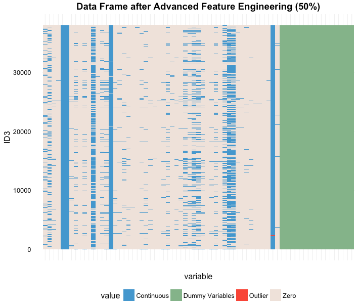
According to the random forest importance selection there are 15 negative, 27 zero, and 71 positive importance features in the dataset. Negative features could hurt and model and zero importance creates no value so we'll cut the dataset down to 71 variables and check our heat map again (same code as above, basically):
Ahhh.....the feature engineering is really starting to look good even if we still have a ton of zeros and a couple of outliers that are nestled into continuous variables. Thumbs up to us.
COMPUTATIONAL EFFICIENCY
One last thing before we jump into the model--let's deploy parallel computing. Most machine learning exercises go through countless iterations to tune and test the results that can last hours so let's use a library(doMC) to setup my laptop to run at top efficiency. I have a 2.6 GHz Intel dual-core i5 with hyper-threading giving me 4 cores. 4 cores vs 2 cores probably won't be a huge difference because there's still just 2 CPUs but we'll max it out and squeeze some more efficiency. I ran a quick test on an abbreviated XGB hyper parameter search (I'll get to that shortly) and here are the results:
Another option would be to access AWS and Google Cloud Computing, both fantastic platforms, in order to boost computational power. I did setup an AWS server with 8 cores and 16 Gb rams and ran a few computations but ultimately went for the free computing power of my laptop. AWS is a fantastic option for on-demand computing power and clustering options.
READY TO MODEL
Given the binary dependent variable, an easy model choice would be a logistic regression. I ran a few basic logistic regression and random forrests but ultimately, and after viewing other Kaggle results, I decided to focus on the XGBoost, a gradient boosting model.
WHY XGBOOST?
Gradient boosting is beneficial in this case because the sparse dataset makes the best use of weak learners by combining them with strong learners through an iterative process into an ensemble. XGBoost is a very popular gradient boosting algorithm that allows for quick tuning, built-in penalty for complexity, and willingness to accept pull requests such as early stoppage and custom loss functions. XGBoost, specifically, includes a formal model complexity regularization function that is intended to prevent over-fitting. Also, the “X” or “Extreme” portion of the library is meant for systems optimization through early stoppage and parallel computing for a scalable, portable, and accurate package.
Read more from the author, Tianqi Chen.
MODEL I: BASIC FEATURING
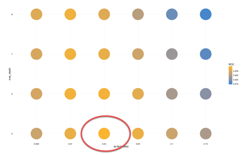
The basic featuring excludes useless variables (all zeros and duplicates) and highly correlated variables. In the end, we'll use a hyper parameter grid search to tune an XGBoost model with 135 independent variables. After several iterations, the below grid ended up having the best results:
The best results for the basic featuring model are:
- max_depth = 5 (number of splits at each leaf)
- eta = .03 (learning rate--lower is slower)
- colsample = .85 (subsample ratio of columns when constructing a new tree)
- gamma = 1 (default)
- subsample = .95 (tested several from .5 to 1. Best results)
- nrounds = 150
Cross Validation
Lets check the cross validation.
That's the basic model. There is a concern of overfitting as you can see the test set really flattens out at about 150 rounds. I ran this several times and received similar results and some results with a larger We'll get to the results in a minute but they were a surprisingly very good!
Now, is the time to test whether all the tricks that tried and the 20% of tricks that actually made a difference really DID make a difference, we'll run a hyper parameter search a few times. Because we narrowed down our dataset to 71 features, this parameter search only took 2.5 hrs rather than 3.5 hrs with basic dataset.
(No need to duplicate code snippets....same setup as the basic featuring but with different a dataset and parameters.)
Like the basic featuring, there is a fair amount of overfitting but not as bad as basic featuring. Still, the advanced featuring results don't quite meet the first model. The final model for advanced featuring:
- max_depth = 4 (number of splits at each leaf)
- eta = .03 (learning rate--lower is slower)
- colsample = .75 (subsample ratio of columns when constructing a new tree)
- gamma = 1 (default)
- subsample = .5 (tested several from .5 to 1. Best results)
- nrounds = 350
Data RESULTS AND CONCLUSION
This dataset was done in conjunction with a modified neural networks model developed by Thomas Boulenger and Anna Bohun. The model and predicted results were submitted to Kaggle and the best, final results are:
In this case, the simplest model won. In full disclosure, the neural nets model is still being tuned and takes a considerable amount time and computational power to tune it just right. That is also a huge benefit to the XGBoost--computational efficiency. Within the Kaggle rankings, the top model received a top 15% ranking; however, the rankings are very flat with .001 differentiating the top 100. This particular dataset holds enough data data to make an easy, off-the-shelf model in logistic regression or decision forms but there are likely sparse data on ~16% of the dataset which makes training and predicting on those observations extremely difficult.
The dataset is prohibitive to attain a score higher than .84 but it goes to show that the problem Santander poses--discovering unhappy customers before it's too late--still shows clarity for 84% of the datasets and is likely enough to draw specific policies or procedures from the importance variables. Santander holds the decoder ring to create those policies and they have all several algorithms if automated products are to be created.


