Higgs Boson Signal Detection
Code: Github
Preface
Discovery of the long awaited Higgs boson was announced July 4, 2012 and confirmed six months later. 2013 saw a number of prestigious awards. But for physicists, the discovery of a new particle means the beginning of a long and difficult quest to measure its characteristics and determine if it fits the current model of nature, which is a daunting endeavor. Therefore CERN, the European Organization for Nuclear Research, in collaboration with the data science competition site, Kaggle, initialized an open source challenge entitled the Higgs Boson Machine Learning Challenge to explore the potential of advanced machine learning methods to improve the discovery significance of the experiment. Our team took on this challenge and with limited backgorund in particle physics, we devised a systematic approach to first understand the dataset, test individual machine learning methods, and then expand on our findings from there.
Understand Dataset
Missing Data
Complete cases in the training data is 68,114 out of 250,000 observations or only 27.2% of the dataset. This is a red flag for handling missing data with imputation because of the overwhelming number of missing data. Since we do not have a very good handle on advanced physics, this meant that we had to rely on using methods that handle missing data well such as XGBoost.
Correlation Plot
The correlation plot shows strong relationships among some of the variables. We can see high correlations between some of the DER(derived variables) with PRI(primary) variables.
Table Plot
The table plot was designed to handle large data sets and is very a powerful visual tool to understand distinguishing factors within each variable and across variables.
The table plot divides the observations in 100 equal groups which are plotted as rows. The mean for each group of observations is displayed as a line and the accompanying standard deviation is displayed as a dark blue bar surrounding the mean.
In the table plot below, the results are sorted by the outcome (“s” or “b”). One can immediately see that in some of the variables the means and/or standard deviations are quite different. The table plot directs us to variables that appear to be the most discriminating in terms of distinguishing whether observations are “signal” or “background”.
Based on the table plot and supported by calculations of mean differentials and standard deviation differentials, we selected a reduced set of 10 variables that we deemed to be the most important predictors and ran them using our model. It is worthy to note that 9 of the 10 variables chosen were DER variables.
Principal Component Analysis
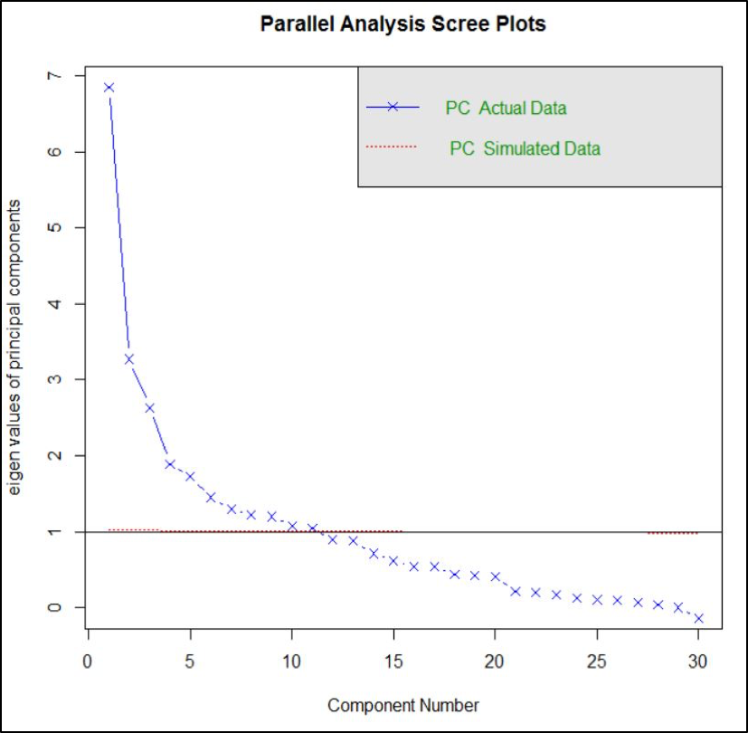
As a part of exploratory data analysis, we employed Principal Component Analysis, an unsupervised method, to determine whether it is practical to reduce dimensions. The first principal component explained only 23% of variance. Based on the result of scree plot, we reduced dimensions to 10 principal components, but even then only 75% variance is explained. PCA showed us that it would be difficult to eliminate variables without sacrificing prediction accuracy.
A Note On AMS, Weights, and Thresholds
Approximate Median Significance (AMS) is the metric by which Kaggle evaluates entries for the Higgs Boson Machine Learning Challenge. In a nutshell, through weights the AMS gives positive points for True positives (predicting “s” when outcome is really an “s”) and gives negative points for False positives (predicting “s” when outcome is really a “b”) except that the negative points for False positives are roughly twice in magnitude than the positive points for True positive. This is the reason why the optimal results for the models use a threshold of around 15% - the threshold being the percentage of “s” predictions out of the 550,000 total predictions submitted to Kaggle for evaluation. Compare 15% to the 34% “s” in the training data and you can see the effect of double penalty for False positives.
Test Individual Models
Random Forest
The first individual model we tested was a random forest as this model is typically quite effective on large datasets, can work with many features, and quickly gives a sense of which variables are most important. We trained this model under the following conditions:
- 250,000 training samples
- AMS rather than accuracy
- 2 fold cross-validation repeated once
- 3 different “mtry” values (2, 16, 30)
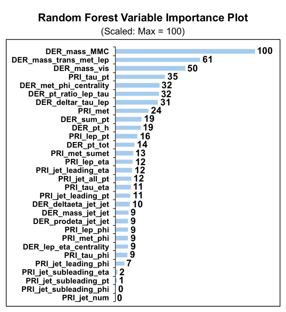
As expected, the variable importance plot below clearly demonstrates the relevance of the mass related variables, particularly the “DER_mass_MMC” feature. This is consistent with findings in the previous section.
Unfortunately, the best AMS score produced on the test data set was 2.10, which is well outside of the top 50% of the Kaggle leaderboard. Given the large gap between the random forest model performance and the top models in the competition we decided to move forward with other individual models rather than continuing to tune the random forest.
Neural Network
After using random forest, we then attempted a more complex model using a neural network. One of the biggest problems with neural networks and most black box methods of prediction is that tuning parameters is often difficult because accuracy does not necessarily improve on a linear scale with tuning. Thus, when constructing the neural network for this data, the choice of network topology and complexity was a pressing concern and we sought to achieve a more systematic approach towards finding the optimal network topology and probability threshold for choosing signal over noise to achieve the highest possible AMS score.
To achieve this, we built a function containing a simple for-loop that creates a neural network model with one hidden layer and an increasing number of hidden nodes for that layer with each iteration. Nested within each one of these node-determining iterations is another loop that then finds the threshold value at intervals of .025 that results in the highest AMS score given the topology set in the parent for-loop. Through this methodology, we were thus able to ascertain the optimal number of hidden nodes on a single hidden layer and its threshold that yielded the highest AMS score.
When testing this function on sample sizes of 10000 and below, this process worked flawlessly and with each increasingly complex network topology the function would pick a different threshold that maximized the AMS score on the sampled training and validation set. However, when using the method on the entire training data, with every iteration of increasing hidden nodes on the single hidden layer, the method would choose the same optimal threshold of 1 and deciding to classify every observation in validation set as background which produced a poor AMS score of .599. So why was this happening? Lets investigate some possibilities...
If you remember back to the section above where we sought to understand the data, we discovered that
- Some of the features are highly correlated
- There would be missingness in some feature data that was often dependent on the existence of another feature having data or not.
- PCA analysis only explained 25% of the variance in the data and even choosing the first 10 principal components only explained 75% of that variance, which both imply that overall data has limited dimensionality and colinear
- The ratio of signal to noise is very skewed
Through these observations on the data, we can hypothesize that there may be complex dependency between highly correlated features that results in classification of finite signal over background and this would thus give an explanation as to why the neural network we engineered performed poorly and always chose to classify the entire data set as background. Because of the potential interdependency between the features theorized above, it is possible that given a single hidden layer topology, the neural network will never encapsulate this complex relationship and therefore always yield a poor AMS score. To remedy this, we may want to in the future try not only optimizing on network for threshold and the depth of a single layer, but through the number of layers chosen in the network topology. Perhaps a wider topology would allow the network to better encompass and tune itself to the inter-dependent relationship between features and thus be a better model of the data and yield a higher AMS score. The next complex model we chose to train on the data was XGBoost.
XGBoost
Before building the model, we subset the training dataset provided on Kaggle into our own sub-training and sub-test. Consider an extremely unbalanced ratio of signal and background counts, we utilized the sample.split() function in R to ensure that both sub-traning and sub-test would have same signal/background ratio. In other words, we avoided a scenario where sub-training might have 85% background while sub-test contained 99% background.
The error of a model can be an effect of bias and variance. We got a mediocre result from random forest, which has relatively low bias and high variance due to fully growing the decisions tress in parallel, thus we moved on with boosting model, where we would have higher bias and lower variance by growing sequential trees.
The xgboost model yielded a pretty good result with default parameters. We then constructed our own cross-validation function to grid search the best tuning parameters for high accuracy and AMS score.
After running 1,050 models, we found the parameters associated with the highest training AMS score are eta = 0.1, max_depth = 9, and nrounds = 85.
The ranking on Kaggle leader board of this submission wasn’t as high as we expected, indicating potential overfitting. By slightly tuning the parameters into eta = 0.1, max_depth = 10, and nrounds = 75, we improved the AMS score to almost 3.7.
This submission ranked us to top 100. The rationale behind this performance advancement was that we improved each individual tree by increasing the maximum depth of a tree and eased the overfitting issue by decreasing number of rounds for boosting.
Takeaways and Next Steps
Takeaways
- EDA indicates that mass related variables are most important
- EDA shows mean and standard deviation indicate that of many variables tend to vary for signal vs background events
- Tuned xgbBoost model yield highest AMS score of our tested models
Next Steps
- Continue to tune neural network model
- Attempt ensemble model given best neural net and xgbBoost models
- Attempt other ensemble model combinations


