Fraud Detection - Detecting Fraud from Customer Transactions
The skills I demoed here can be learned through taking Data Science with Machine Learning bootcamp with NYC Data Science Academy.
Project Code | Linkedin | Github | Presentations | Email: fredchengnyc@gmail.com
Data Description
The data comes from real-world e-commerce transactions from Vesta, a leading payment service company, and contains a wide range of features from device type to product features.
The task of this competition is building machine learning models to predict the probability that an online transaction is fraudulent, as denoted by the binary target isFraud.
After merging the provided datasets, we got one large-scale train dataset to manipulate, which contains 590,540 rows and 434 features.
The features of data have been completely anonymized for privacy, given only a minimal explanation by the data provider - Vesta. So we have to build models with more discovery on features' meaning and judgment calls. Click here to check the introduction to the features.
Business Understanding
As a data scientist, we have to understand business problems and requirements to convert them into machine learning problems and goals before diving into exploratory analysis and predictive modeling:
- Flag fraudulent transactions while also avoid misclassifying legit transactions as fraudulent - Build predictive models to tackle a binary classification problem minimizing both false negatives (FN) and false positives (FP).
- Be cautious about large transactions, as they can make a greater loss - Set a lower and thus stricter probability threshold of classifying a transaction as a fraud when involving a higher transaction amount, vice versa.
- Detect fraudulent transactions immediately - Build models with both low running time and good performance. LightGBM can be a good fit.
- Understand what factors are more predictive to detect fraud; thus, they can be investigated further and more relevant data can be collected - It’s important to not only focus on performance, but also inferences; simple models with better interpreting power also have crucial roles.
- Balancing convenience with security. According to a recent Fiserv analysis of 20 million cardholders, if a person has two or more legitimate transactions denied within a seven-month period, the average spending on that card six months after the last denial goes down 15 percent. What's more, 20 percent of people will stop using the card completely.
- "It's critical that you balance the automated measures with exceptional customer service," explained- Vince Liuzzi, chief banking officer at DNB First. The level of service might be enough to offset any annoyance with having to verify purchases or deal with a temporarily locked card - Optimizing metrics concerning both FP and FN like AUC ROC, F-beta, and lift scores.
Exploratory Data Analysis
I discovered basic statistics, distributions, missingness, business insights, removed outliers and useless features, and created new features in this section.
As there are too many features to present in the blog, I will only display the features with meaningful findings. For my complete project code and analysis, click here.
(See more details in "Attachments - Extra Details of EDA" at the bottom of the page)
Detecting Missing Value
After importing and merging the datasets, I firstly took a look at the missingness. As you can see from the plot below, the dataset has a large portion of missing value and this occurred in 411 features of the total 433 features. Over 47% of features have more than 70% missing value. I removed 9 features because they were missing 99% of the value."
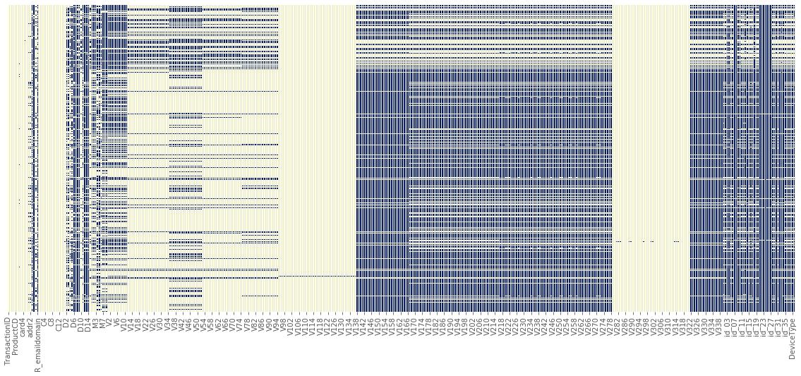 Also, I removed the feature V107 as it has only one unique value in the test dataset.
IsFraud - Target Distribution
As shown in the plot below, the target distribution is extremely imbalanced; only 3.5% of transactions are fraudulent in the training set. An imbalanced data set will lead algorithms to get good results by returning the majority class, which performs badly in predicting test data. That will be a problem, as we are more interested in the minority class. So I performed balancing techniques on the training dataset to force the algorithm to give more weight to the minority class and carefully selected evaluation metrics. They will be discussed in the following sections.
TransactionDT - Timedelta from a given reference DateTime
(see more details in "Attachments" at the bottom of the page) 'TransactionDT' is an important time-related feature that has been masked by large sequential numbers. As its value ranges from 86,400 to 15811131, it's reasonable to infer that the real value is in seconds. Therefore, we can create new features such as hours in a day and days in a week to provide more explicit information to our model. Now let's visualize the new hour and day features from the plot of the frequency of transaction versus the fraction of fraud in different hours:
We can see that the fraction of fraud from 4 am to 12 pm is significantly higher than during the other hours, with the highest fraction occurring from 7 pm to 10 pm. In contrast, the lowest fraction of fraud occurs from 2 pm to 4 pm. It tells us that there is a reversed trend between transaction frequency and the fraction of fraud, which makes sense because scammers can put through unauthorized charges when people are sleeping and not likely to notice, right away.
Based on this inference, we can create a new feature on both train and test datasets:
- Setting hours larger than 7 and smaller 10 as 'high warning signal,'
- hours smaller than 14 and 16 as 'lowest warning signal',
- hours larger than 4 and smaller than 7, and hours larger than 10 and smaller than 14 as 'medium warning signal',
- and the other hours as 'low warning signal.'
The 'hour' turns out to be a highly important feature in prediction.
TransactionAmt - Transaction Amount
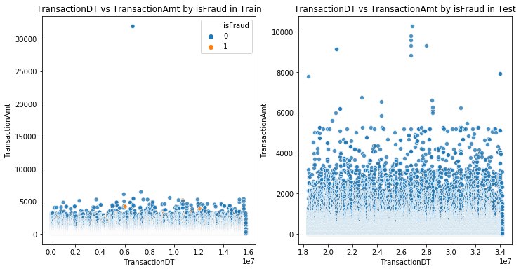
The transaction amount is another vital feature that gained high feature importance to investigate. It has no missing value. Let's visualize it in both train and test datasets by scatter plots:
As we can see from the left figure above, two extreme outliers are found duplicated with a value of $31,937 in the training set. Outliers like this can cause an overfitting problem. For instance, the tree-based models can put these outliers in leaf nodes, which are noise and not part of a general pattern. Therefore, I decided to remove the values larger than 10,000 in the training set. However, we can't remove any rows in the test set as Kaggle requires to submit a prediction result that matches the original length of the test set.
I also removed outliers in many other features in the same way above.
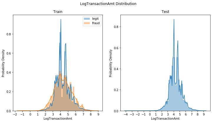
Due to the skewness of the transaction amount, I also created a new feature by taking a log of it. Here is the distribution plot after the log transformation:
It seems that the transactions with 'LogTransactionAmt' larger than 5.5 (244 dollars) and smaller than 3.3 (27 dollars) have a higher frequency and probability density of being fraudulent. On the other hand, the ones with 'LogTransactionAmt' from 3.3 to 5.5 have a higher chance of being legit.
'V1' - 'V339' - Vesta engineered rich features, including ranking, counting, and other entity relations.
The 339 features in V1 - V339 is intimidating, as they are all 'encrypted' and boost the dimensionality. Instead of getting into details, I checked the pairwise correlation through a heatmap below. As most features are correlated with each other, I performed a PCA on the V features that can not only mitigate the curse of dimensionality but also save tons of running time, as well as decorrelate the features to improve model performance. The downside of PCA is that we will lose the interpretation of the features. But it's not a big deal since the meaning of these V features is unknown anyway.
Data Preprocessing
Additional Feature Engineering
Except for the feature engineering we have done alongside the EDA above, now we can do extra feature engineering by using some group statistics, scaling, standardization, and aggregations of top features generated by default LightGBM model, providing our models more information by determining if a value is common or rare for a particular group and disclosing more of the relationship between the top features.
Label Encoding, Missing Value Standardization, and Dimensionality Reduction(PCA) on V features
As we will use tree-based models that are capable of handling categorical variables, we only did label encoding to all the categorical variables. After that, we performed PCA to compress V features into 30 principal components, as they have explained around 98.6% of the variance.
Then we standardized all the missing values by -999, which is a negative number lower than all non-NAN values since tree-based models are robust in handling missing value and will treat these -999 numbers as a special category, given the same attention as other numbers. In addition, we also convert infinite numbers Inf to NaN.
Data Splitting
The last thing we do before modeling is to split our data into a 70% training set and a 30% validation/testing set, which acts as unseen data.
Apart from the splitting above, I also split the training and validation set based on the log transaction amount as transactions have different levels of cost (because TransactionAmt is highly skewed):
- High-cost set: The transactions with Log transaction amount one standard deviation above the mean - Transaction amount larger than $530; 14602 observations in train.
- Medium-cost set: The transactions with Log transaction amount within one standard deviation above and below the mean - Transaction amount larger than $12 and smaller than $530; 390613 observations in train.
- Low-cost set: The transactions with Log transaction amount one standard deviation below the mean - Transaction amount smaller than $12; 7366 observations in train.
- Let's called them "Transaction cost-based sets."
I trained models on these sets using different metrics and select thresholds that maximize the corresponding scores. The business implementation varies according to the cost and predicted probability as well. We will talk about it.
Tackling Imbalance Data
As discussed in the EDA - target distribution, we are handling a typical extreme imbalanced dataset, which requires us to implement balancing techniques. There are multiple balancing techniques in both oversampling and downsampling. Since downsampling would make us lose tons of rows and information for the extreme imbalance (3% minority class). I only considered oversampling techniques, including using the argument class_weight="balanced" in Sklearn and SMOTE.
The class_weight="balanced" basically replicates the smaller class until having as many samples as in the larger one, in an implicit way, so that the model can penalize mistakes it makes in the minority samples. The idea is to force the model to give more weight to the minority class.
Before this complete and self-improving project, I also did this competition in a simplified version cooperating with other fellows. We used the technique of oversampling the minority class along with SMOTE, which stands for the Synthetic Minority Oversampling Technique. It judges nearest neighbors based on Euclidean distance between data points. Here is a simple visual example:
 I also want to share a vital practice I learned about the upsampling technique that we need to be cautious:
We should do upsampling in each training fold in the cross-validation instead of performing it before the cross-validation.
If cross-validation is done on already upsampled data, the scores don't generalize to new data (or the test set). To understand why this is an issue, consider the simplest method of over-sampling, which simply copying the data point. One instance is of every data point from the minority class being copied 6 times before being split. If we do a 3-fold validation, each fold has (on average) 2 copies of each point.
If our classifier overfits by memorizing its training set, it should be able to get a perfect score on the validation set. Our cross-validation will choose the model that overfits the most. We see that CV chose the deepest trees it could.
In addition, we should never perform oversampling before the train-test split as it would cause a destructive data leakage problem. It's like students (models) taking the exam but knowing answers to most questions already, which is called data leakage. Although SMOTE is not a naive upsampling method and will mitigate this issue, we do can run SMOTE before the cross-validation, the cross-validation score would still be over-optimistic.
In real practice, we can use a pipeline from the imblearn library to execute the SMOTE within cross-validation automatically. However, running it can be very costly in terms of time e since we need to perform SOMTE, which is time-consuming itself, together with every model training that usually comes with a highly time-consuming grid search. So after doing some experiments with a small-size sample, I decided to use class_weight='balance' argument method instead due to the crazy running time. Here is an excellent blog with experiments about this topic that you can look up to.
Model Selection Criterion and Evaluation Metrics
Since we are facing a binary classification problem on an extremely imbalanced dataset, the confusion matrix and a series of derived measures are essential tools to check the performance of our models. But we need to choose the model selection criterion very carefully. The commonly used measure Accuracy can't be used in this case as it would be easily masked as a satisfying score by classifying all the cases to the majority class.
Data scientists have to solve problems with a business mindset. Although this Kaggle competition uses the AUC ROC score to evaluate models, in the real business world, we have to choose the metrics under the business context. So let's analyze what metrics to use:
What we are primarily concerned with in the confusion matrix are TP (the number of True Positives: model correctly predicts fraud), FP (the number of False Positives: model incorrectly predicts fraud), and FN (model incorrectly predicts legit transaction). We aim to minimize both FN and FP and maximize TP because FN would cause direct pecuniary loss from undetected fraud as well as negative customer experience, and FP would cause customers' dissatisfaction by making them feel embarrassed and worried. That could induce a churn, which is an indirect loss.
So we want to minimize both of them. We also want to maximize TP, as it correctly detects fraud in the covert minority class and thus stops loss. Therefore, the measures that are appropriate to use as the model selection criterion regarding these business considerations are precision, recall, f-beta (like f1, f2, f0.5), and AUC ROC score.
ROC curve plots the true positive rate on the y-axis versus the false positive rate on the x-axis as a function of the model’s threshold for classifying a positive. AUC stands for the area under the ROC curve. The higher the AUC score, the better our model's overall performance. AUC ROC gives consideration to all quadrants in the confusion matrix. However, we care much less about TN.
To put emphasis on FP, FN, and TP, recall, and precision usually come into play. However, like Accuracy, using recall and precision solely can be dangerous. Recall identifies the rate at which observations from the positive class are correctly predicted; precision indicates the rate at which positive predictions are correct. But if we label all transactions as fraud, then our recall goes to 1.0.
And if we only identify a single transaction correctly, the precision will be 1.0 (no false positives). However, our recall will be very low because we will still have many false negatives, which is a trade-off in the metrics we choose to maximize, like when we increase the recall, we decrease the precision.
Therefore, I used F-beta, where the beta parameter determines the weight of recall in the combined score, to combine the two. Then I tuned the beta (not a hyperparameter) according to our business need for finding the best model.
I split data into high, medium, and low cost sets based on the log transaction amount. I presume that the cost of incorrectly predicting fraud as legit (FP / low recall) in high-cost transactions is higher than incorrectly predicting legit as fraud (FP / low precision).
Similarly, the frustration for getting blocked when spending 5 dollars buying a burger standing on a long line may outweigh the potential benefits of preventing a small unauthorized charge. That's why we need to use different criteria. Therefore, I used the F2 score; twice the weight is given to recall as opposed to precision, as the scoring in the grid search cross-validation on the high-cost set to select the best model, F1; same weight given to recall against precision, on the medium-cost set, and F0.5, which gives twice as much weight to precision, on the low-cost set.
I built Decision Tree, Random Forest, and LightGBM models on the whole training set using the AUC ROC score and built LightGBM on Transaction cost-based sets using F-beta.
To better illustrate the performance from a business perspective, I also used Cumulative Gains Curve and Lift Curve. To understand them, you can look up here.
In addition, we will discuss the decision of the thresholds to use after tuning the models using different criteria as well as the corresponding possible business implementations.
Modeling
In the modeling part, I used three algorithms: decision tree, random forest, and light gradient boosting machine.
Modeling in the whole training set using 'AUC ROC' score as model selection criteria
Decision Tree
We build decision tree models firstly as both a benchmark of the following models and the simplest model with relatively strong interpretability. A decision tree was built with default hyperparameters in the first place.
I got a purely overfitting model with training AUC score 1.0 and testing AUC score 0.75 as well as a big number of leaves - 11377, and deep depth - 76. So I tuned it using a randomized grid search with stratified cross-validation using 'AUC ROC' as scoring and hyperparameters used to restrict tree size and prune the tree with minimal cost-complexity. (check my project code to see all the grids I used)
The randomized search was set with 60 iterations in terms of a rule of thumb: with 60 iterations 95% of the time, the best 5% sets of parameters can be found, regardless of grid size.
I got a tree with the least overfitting. The AUC score results on the training are 0.819 and the test is 0.818. The number of leaves of the tree is 9 and the depth is 4, much smaller than the base tree while returning us a higher testing score.
The smaller decision tree is easier to present and interpret. Here’s the visualization:
This tree diagram would be more powerful in interpretation if the features' meaning is not masked.
Feature importance:
Random Forest
Applying the same procedure as above, we firstly built a random forest model with default hyperparameters as the base case and the result I got is AUC score 1.0 in the training and 0.934 in the test, which is overfitting. So we tuned the model in the same way as the decision tree and we got a much less overfitting model that results in AUC score 0.90 in the training and 0.89 in the test.
We got the identical feature importance to the decision tree:
LightGBM - Final Model
LightGBM is a high-end complex model that outperforms many others in Kaggle regarding its performance and speed. The similar tuning strategies above were applied.
The default LighGBM results in AUC score 0.946 in the training and 0.926 in the test. The feature importance of default LightGBM was used as a reference to perform feature engineering and selection.
Even the base case of LightGBM results in a significantly improved score.
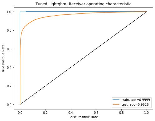
After tuning with 200 iterations in a randomized search, we got a little overfitting but overall improved model with 0.9999 AUC score in the training and 0.9625 in the testing, which is quite good. Let's visualize the AUC scores in both training and testing:
To select a threshold applied in unseen data, let's extract the testing score and visualize the trade-off between True Positive Rate/Recall and False Positive Rate with thresholds changing on the right y-axis:
As shown above, we can select a higher threshold to gain a better True Positive Rate/Recall, or a lower threshold to gain a better False Positive Rate. The selection strategy is based on business needs. I used the transaction amount as a benchmark to select while it is only one of the options.
According to the Lift Curve and Cumulative Gains Curve below, we can draw the conclusions:
If we contact only 10% of the transactions’ account owner then we will detect 88% of the total fraudulent.
In other words, by checking only 10% of transactions based on the predictive model we will detect 9 times as many frauds as if we use no model.
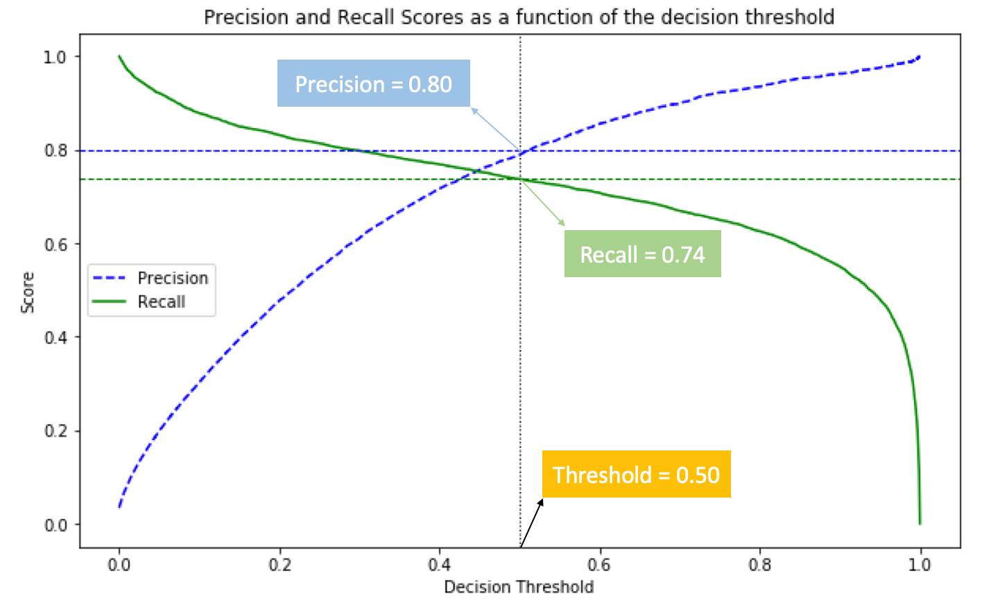
Selecting the decision threshold to 0.5, we got a 0.74 recall and 0.80 precision score. This indicates that the probability of our model to detect all the fraudulent transactions was 0.74 (recall) and the probability that all the detected fraudulent transactions were fraudulent is 0.80 (precision).
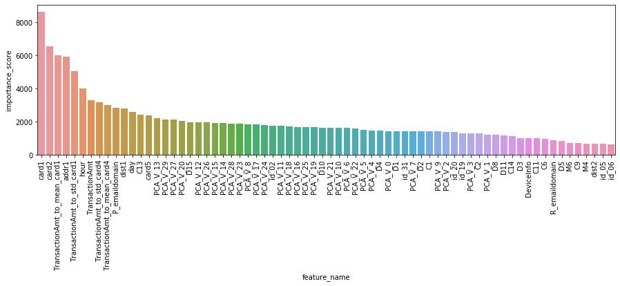
Feature importance:
Given the feature importance of the final model above, we can see that the features about Payment Card Information, address, transaction time, distance from address, Email Domain of Purchaser, and engineered features by aggregations of top features are most predictive to detect fraud.
We can also perform feature selection by removing the variables with feature importance smaller than a threshold.
LightGBM on Transaction Cost-Based Sets
Now we build LightGBM models on the "Transaction cost-based sets". I used F-beta as the model selection criterion in randomized grid search cross-validation with the same gird on the three sets.
Low-cost set using F0.5 score
The low-cost set has 7,366 observations, which is the least. The best threshold of the F0.5 score in the test is 0.76, and the corresponding score is 0.90, which is the highest score among the three sets.
Setting threshold as 0.76, we got a 0.70 Recall and 0.9686 Precision score on transactions smaller than 12 dollars.
The performance of this model is fairly good. It has a nearly perfect probability (97%) that all the detected frauds were fraudulent and a nice probability (70%) to detect all the fraudulent transactions.
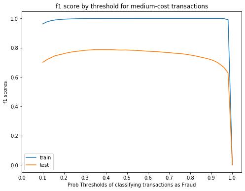
Medium-cost set using F1 score
The model is severely overfitting. In the future work, I will train simpler models and carefully tune them on larger data size of large transactions, so as to the medium cost transactions.
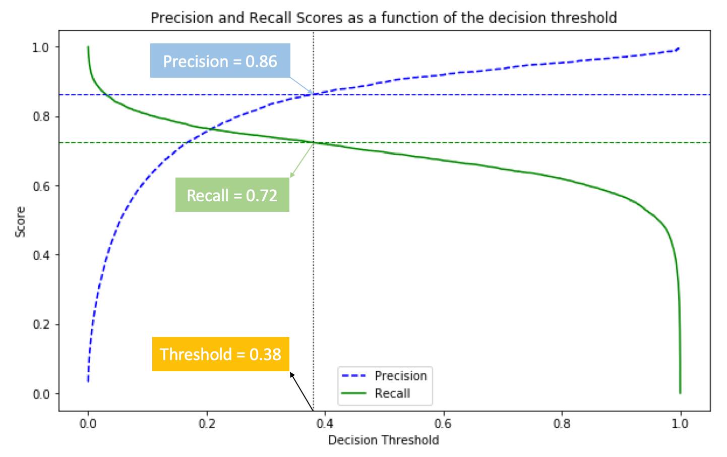
The medium-cost set has 390,613 observations, which is the most. The best threshold of the F1 score in the test is 0.38, and the corresponding score is 0.79.
Setting threshold as 0.38, we got a 0.72 Recall and 0.86 Precision score on transactions larger than 12 dollars and smaller than 530 dollars.
The recall and precision are more balanced in this range of transaction amounts.
High-cost set using F2 score
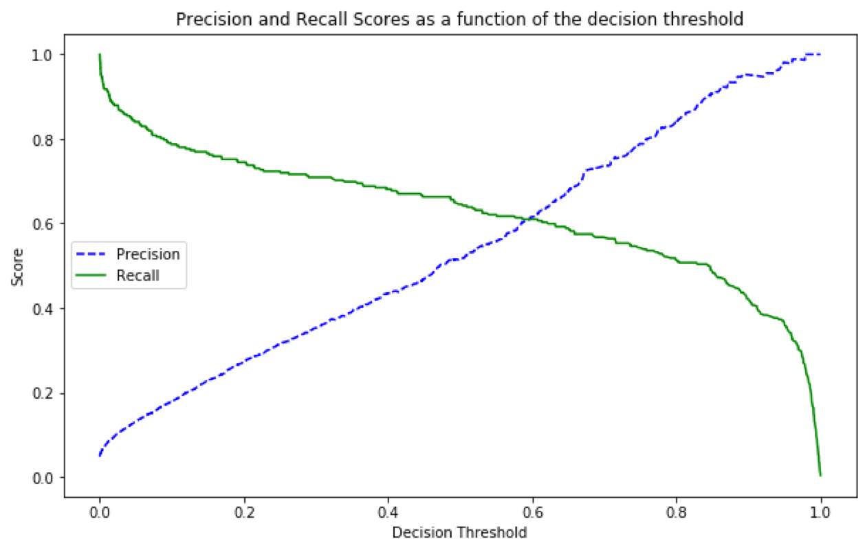
The best threshold of the F2 score in the test is 0.49, and the corresponding score is 0.67. As the High-cost set only has 14,602 observations in the training, having more samples might generate a much better prediction.
Setting threshold as 0.49, we got a 0.66 Recall and 0.52 Precision score. Theoretically, we can move the threshold to the left to gain higher recall on large transactions. But this will make precision decrease a lot for its large slope. The overall performance of this model is not very satisfactory and it will be improved in future work.
Business Implementation:
In practice, we need to combine machine learning and automation with direct customer contact to identify and address potential fraud. Our models should trigger a follow-up action like a text message, notification on cellphone application, or phone call to the customer.
Here is my simplified hypothetical implementation strategy based on models' predicted probability and transaction amount with assistances from customers:
| High probability being a fraud | Low probability being a fraud | |
| High-cost transactions | Block and confirm | Let through and confirm |
| Medium-cost transactions | Let through and confirm | Let through and flag risk on application |
| Low-cost transactions | Let through and flag risk on application | Let through and flag risk on application |
Customer education is also vital to defense against traditional scams like Phishing which is still effective.
According to the U.S. News interview with Vince Liuzzi, chief banking officer at DNB First, while automated systems are doing the bulk of the work to detect fraud, financial institutions are hoping customers will help as well. Tools that enable that include searching an extended account history online to let people easily find questionable transactions, or giving customers greater control over the use of their card, like sending alerts when cards are used, letting customers lock down a card to a certain geographic area and "turn off" cards they won't be using.
References:
-
- https://www.datascienceblog.net/post/machine-learning/specificity-vs-precision/
- https://medium.com/@gtavicecity581/ieee-fraud-detection-469398ce1ac4
- https://nycdatascience.edu/blog/student-works/kaggle-fraud-detection/ (I was one of the contributors)
- https://www.kaggle.com/cdeotte/eda-for-columns-v-and-id
- https://www.kaggle.com/c/ieee-fraud-detection/discussion/108575
- https://www.kaggle.com/kabure/extensive-eda-and-modeling-xgb-hyperopt/notebook#Some-feature-engineering
- https://www.kaggle.com/artgor/eda-and-models#Feature-engineering
- https://money.usnews.com/banking/articles/how-banks-are-working-to-protect-you-from-fraud
Attachments - Extra Details of EDA
'P_emaildomain' and 'R_emaildomain' - Email Domain of Purchaser and Recipient
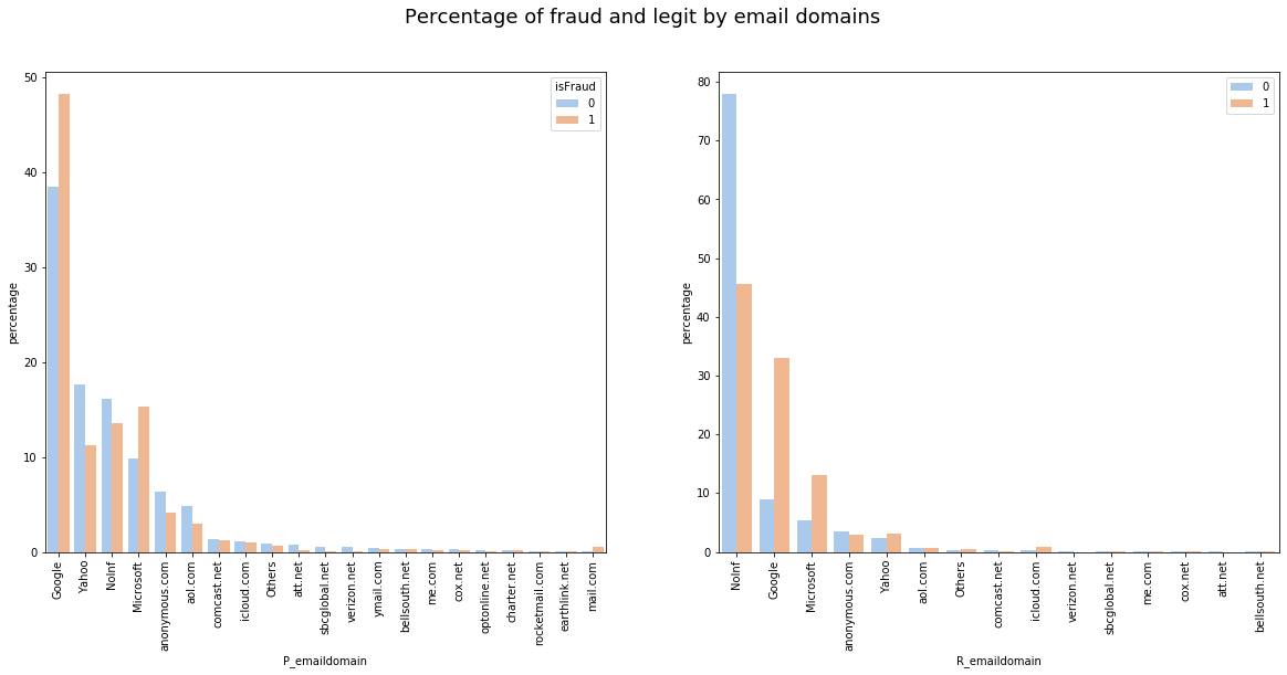
P_emaildomain is another crucial feature with high feature importance scores to analyze. It represents the email domain of the purchaser in transactions, while the R_emaildoamin represents the recipient's domain.
Apart from the splitting strategy mentioned above, I also transformed features with similar observations/strings by grouping them. For example, observations 'yahoo.com' and 'yahoo.com.mx' are grouped as 'Yahoo'. Besides, all the values with less than 500 entries are set as "Others" and all missing values are filled by 'NoInf.'
After the transformation:
Card3 - Masked Payment Card Information
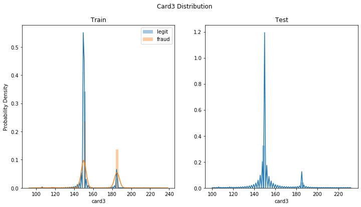
Apparently, card3 is a categorical variable, although it's numerical. As the values around 150 have higher chances of being legit; and the values around 180 are more likely to be, we can create another new feature that categorizes card3:
- If the value is larger than 160, then 'Positive‘.
- Otherwise 'Negative'
Card6 - Masked Payment Card Information
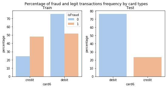
In feature card6, there only 15 observations are 'charge card,' and 30 observations are 'debit or credit card' in the training set but not in the test set. As the sample size is not sufficient for finding a general pattern, and the majority card6 type is debit, we can replace the observations with these values to 'debit'.
After the replacement:
'Addr1' and 'Addr2' - Masked Purchaser Billing Region and Country
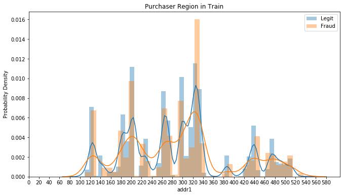
Another important feature with the high feature importance from our final LightGBM model is 'addr1.' It refers to the purchasers' billing region, which distributes in around 300 distinct values/regions. As we can see from the plot below, region 330 has a higher frequency of fraudulent transactions than the other regions, as well as the highest transaction frequency in total. We can do more analysis by collecting more information about it once knowing the real feature meaning.
In the 'addr2' feature, there are around 70 billing countries, and the country 87 accounts for around 88% of transactions. Since the data provider, Vesta is mainly based in the United States, 87 likely represents American accounts.
'id 30' - Operating System
I created new columns by parsing divisible strings, such as separating 'Windows 10' into the operating system 'Windows' and the version '10'. This splitting strategy is also implemented in other features.
TransactionDT - Timedelta from a given reference DateTime
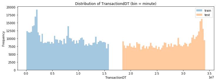
'TransactionDT' is an important time-related feature that has been masked by large sequential numbers. As its value ranges from 86,400 to 15811131, it's reasonable to infer that the real value is in seconds. By calculating it as seconds, we can see that the training and test datasets are in a different time span. The period of the training and test datasets are 182 and 183 days, respectively.
The total period is 395 days, with a 30 days time gap between train and test, shown as the distribution graph below. Therefore, we can create new features such as hours in a day and days in a week to provide more explicit information to our model. But we don't want to create a feature of months in a year because we only have one-year data, which makes it impossible to find patterns between months in years. We may also consider splitting the data by the time order.
'Dist1' and 'Dist' - Masked Distances from Addresses
For the feature 'dist1,' I found that its mean value of fraudulent transactions is 1.5 times higher than of legit transactions. I guess that's because scammers tend to illegally swipe the card in a longer average distance from the cardholders' address. As you can see in the plot below, I removed the extreme outliers where values are larger than 6000 in the train set, so as the observations larger than 8000 in 'dist2'.


