Guided Procedure to Improve Models in Kaggle Competition
The skills the authors demonstrated here can be learned through taking Data Science with Machine Learning bootcamp with NYC Data Science Academy.
How to Improve Regression Model Accuracy
Kaggle competition has been very popular lately, and lots of people are trying to get high score. But the competitions are very competitive, and winners don't usually reveal how approaches. Usually, the winner just write a brief summary of what they did without revealing much. So it is still a mystery what are the approaches available to improve linear regression model accuracy.
This blog post is about how to improve model accuracy in Kaggle Competition. I will be sharing what are the steps that one could do to get higher score, and rank relatively well (to top 10%). This blog post is organized as follows:
- Data Exploratory
- Numerical Data
- Categorical Data
- Model Building
- Linear Regression
- Lasso Regression
- Ridge Regression
- Data Transformation
- Random Forest
- Gradient Boosting Machine
- Neural Network
- Stacking Models
1.1 Data Exploratory
First, we take a quick look at the data. There are 14 continuous (numerical) features. Surprisingly, the data is fairly clean. Looking at the 2 images below, if we focus on the mean and std, we will realize that mean is around 0.5 and std is roughly 0.2. This means this data may have been transformed already.
Next, we will make histogram plots for all 14 continuous features. What we want to notice here is feature 'cont7' and 'cont9', which are skewed left.
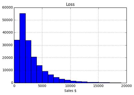
The loss variable (target) did not plot well, so we make a separate histogram plot for loss variable. We realize loss is also skewed left.
To find out how skewed are our variables, we calculate the skewness, and 'cont7', 'cont9', and 'loss' are the 3 variables that are the most skewed.
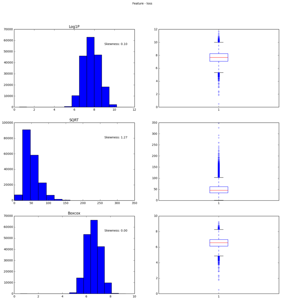
If we further make a boxplot, we can once again see that 'cont7' and 'cont9' have a lot of outliers. If we try to fix the skewness, we might be able to lower the number of outliers.
Here, we will try 3 types of transformation, compare them, and see which one does the best job: log, sqrt, and Boxcox.
We can clearly see the Boxcox worked on all 3 cases, however, we cannot use Boxcox on 'loss' variable, because currently in Python, there is no function to undo Boxcox. So, if we want to transform 'loss' back after prediction to calculate mean absolute error, we will be unable to do that. We will use log later as our transformation for the 'loss' variable.
1.2 Categorical Features
For categorical features, We can make frequency plots. Few major points about the categorical features are:
- Features 'cat1' to 'cat72' have only two labels A and B, and B has very few entries.
- Features 'cat73' to 'cat108' have more than two labels
- Features 'cat109' to 'cat116' have many labels.
Here are some sampled frequency plots to confirm the above 3 points:
2.1. Model Building - Linear Regression
Now that we have our continuous and categorical features analyzed, we can start building models. Note that this dataset is very clean, no missing data at all! What we will do here is to set up a working pipeline and start feeding in raw data first. Then as we do different transformation on the data, we can then compare the new model to our baseline model (raw data case) . Our raw data case will be un-transformed continuous features + dummy encoded features. We have to at least do dummy encoding on the categorical data is because sklearn models do not allow strings in the observed data.
We will fit a linear regression as follows:
As shown above, testing score is much larger than training score. This means we are overfitting the training set too much. A note on the evaluation is that we are using mean absolute error, and it's negative here is because sklearn made it negative so that as we our lowering the error (tuning the model to make the error closer to zero), it looks like we are increasing the score (i.e. -1 - (-2) = 1, so the new score has improved the old score by 1).
2.2 LASSO Regression
It is obvious that we need a regularizer here, so we will use LASSO regression. Remember, LASSO is just linear regression + a regularizing term. We can see below with a 5 fold cross validation, we get cross validation score around 1300, which is close to our previous linear regression score of 1288. We are on the right track here! Note the grid search below tells us the best alpha is 0.1, although the 3 different cases yielded very close result.
2.3 Ridge Regression
Another easy to use regularization is ridge regression. Since we already know that LASSO regression worked well, so this data set is likely to be a linear problem, we will use ridge regression to solve it as well.
The cross validation here tells us that alpha=1 is the best, giving a cross validation score of 1300.
2.3.1 Data Transformation
We have the working pipeline setup now, so we will be using ridge regression to test different data transformation to see which one gives the best result. Remember previously we did boxcox transformation on features 'cont7' and 'cont9', but we haven't really implemented it (we used raw continuous features + one hot encoding categorical features until now). So we will implement the transformation now!
We will implement compare these transformations:
- Raw (numerical/continuous features) + Dummy Encode (categorical features)
- Normalized (num) + Dum (cat)
- Boxcox Transformed & Normalized (Num) + Dum (cat)
- Box & Norm (num) + Dum (cat) + Log1 (Loss variable)
Below is the table comparing side by side the cross validation error. We found that taking log of the loss (target) variable yielded the best result.
|
Raw(num) + Dum(cat) |
Norm(num) + Dum(cat) |
Box / Norm (num) + Dum(cat) |
Box / Norm (num) + Dum(cat) + Log1p(loss) |
|
|
Ridge Regression CV MAE |
1300 |
1300 |
1300 |
1251 |
2.4 Random Forest
Now we have our transformation under our belt, and we know this problem is a linear case, we can move on to more complicated model such as random forest.
Immediately, we see an improvement of the cross validation score from 1251 (from ridge) to 1197.
2.5 Gradient Boosting Machine
We will take another step further to use a more fancy model called gradient boosting machine. The library is called extreme gradient boosting, as it optimizes the gradient boosting algorithm. Here, I will share the optimized hyperparameters. Tuning xgboost is an art, and time consuming, so we won't be talking about it here. A step by step approach is described in this blog post. I will just outline the general steps taken here:
- Guess learning_rate & n_estimator
- Cross validate to tune for min_child_weight & max_depth
- Cross validate to tune for colsample_bytree & subsample
- Cross validate to tune for gamma
- Decrease learning_rate & tune for n_estimator
Using these parameters, we were able to get cross validation score of 1150. Another improvement!
2.6 Neural Network
We will use also use neural network to fit this dataset. It's almost impossible to win a competition now a day without using neural network.
The main problem with neural network is that it's very hard to tune, and it's hard to know how many layers and how many hidden nodes to use. My approach was to start with a single layer first and use twice the number of features as the number of hidden nodes. Then I slowly add more layers. Finally, I obtained the following structure. I used Keras as front end, and Tensorflow as backend. In this model, I got 1115 cross validation score.
So, comparing different models:
| Ridge | Lasso | Random Forest | Gradient Boosting Machine | Neural Network | |
| 5 Fold CV MAE | 1251 | 1263 | 1247 | 1152 | 1130 |
2.7 Stacking Models
Remember, we started out with MAE score of 1300? We've improved it by 14% down to 1115. However, single model is not able to get you good ranks on Kaggle. We need to stack models.
The idea behind stacking is to take the best part of each model where it performs well. An extended guide and explanation is described in this blog post.
A simplified version is as follows:
- Split training set into several folds (5 fold in my case)
- Train each model in the different folds, and predict on the splitted training data
- Setup a simple machine learning algorithm, such as linear regression
- Use the trained weights from each model as a feature for the linear regression
- Use the original train data set target as the target for the linear regression
To make it easier to understand the above steps, I constructed the following table:
| Linear Regression | Column 1 | Column 2 | ... | Target Variable |
| Row 1 | Model 1 Trained Weight 1 | Model 2 Trained Weight 1 | ... | Original Train Data Target, y1 |
| Row 2 | Model 1 Trained Weight 2 | Model 2 Trained Weight 2 | ... | Original Train Data Target, y2 |
| ... | ... | ... | ... | ... |
My code for stacking is in this github repository. I stacked 2 best models here: xgboost + neural network.
Upon submission of my stacked model, I obtained test score of 1115.75
Looking at the leaderboard, 1115.75 ranks about 326 out of 3055 teams if I had submitted before the competition ended. You can verify using this Kaggle leaderboard link. This is roughly top 10~11%.
The code for this blog post is here.


