IOWA Housing Market Price Predictions - Machine Learning
Introduction
For this Machine Learning project, our purpose was to create a predictive model for housing prices in Ames, Iowa. The dataset was provided by Kaggle (the completed information that can be found here: https://www.kaggle.com/c/house-prices-advanced-regression-techniques). Originally, this dataset was made by a professor, Dean de Cock at Truman State University as a class project. Now the dataset has grown in popularity and it is the basic entry level for a highly frequented Kaggle training competition. It has 79 explanatory features to help describe houses and the surrounding properties ranging from square footage to more subjective or categorical features such as quality or garage type. Our team of two set off to explore the dataset, draw inferences statistical analysis and ultimately create a model to predict the correct price of a home in Ames.
1. The Data:
We have about 2900 observation total with 79 numeric and categorical variables; split evenly between training and test datasets. Our dependent output variable is sales price. There are missing data, outliers, and some skewed variables. We need to fix these problems before we can have strong models.
First, let us have a look at the distribution of the response variable, sale price. We can see from the figure that the distribution of sale price is right skewed. The Y-axis represents frequency of the sale price and the transformed normal distribution in first graph while the second graph represents the original skewed data distribution .
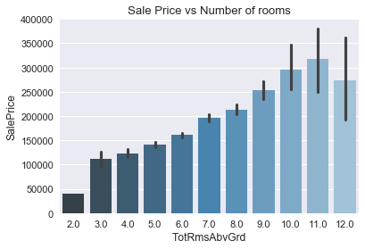
Next, we plotted scatterplots and bar chart to show sale price versus different variables. For example, on this sale price versus total basement in sq feet and number of rooms, it seems that there is a strong positive correlation between variables and sale price.
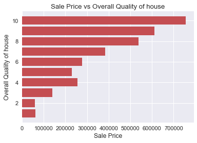
On the Bar Chart of sale price versus overall quality, we have another strong correlation. However, when we take a closer look, the sale price actually increase exponentially as the overall quality increases.
On the correlation plot, we can see that first floor square feet is highly correlated with total basement square feet and garage living area is highly correlated with total rooms above grade. In the feature engineering, we will address these issues.
In addition to some of the EDA and transformations above, the team removed several high price outliers and added some features such as above grade living area square feet.
2. The Models
For the models, we chose a variety of different base models such as Lasso and Ridge regression, XGBoost, and Random Forest.
The first models that we used were the linear models (Lasso, Ridge). The reason why we used these were that they are relatively simple to implement and do not take that long to optimize. We used Ridge because we wanted to minimize the effect of weak predictors for the House's sale price (the target), but not eliminate them because they might provide some explanatory power in the model. We also used Lasso in order to drop unnecessary columns that might not provide any explanatory power in our model. The one drawback for this model is that these models assume a linear relationship to the target, which was not always the case. Another drawback is that these models suffer from multi-colinearity, which can make the estimates for our coefficients inaccurate if they are highly collinear.
After we implemented the linear models, we also implemented the tree based models, such as Random Forest and XGBoost. For this post, we shall separate them into two different segments, Random Forest and XGboost model.
The reason why we included the Random Forest model is because it tends to not over-fit the training set because each decision tree is limited to a number of factors. Although each individual decision tree might over-fit the data, all of the trees can be ensembled together to make a stronger predictor. This can be done because all of the individual trees are uncorrelated. As long as we have enough trees in the Random Forest, the 'noise' of each tree will be averaged and the trend from the strong predictors will stand out. Another benefit from this model is that it does not assume a linear relationship between the variables and the target. One con of this model is that the accuracy of the model can suffer when predicting on data that it has not seen before. The reason for this is because there are only a certain number of leaf nodes, so that means there can only be a certain number of predicted prices. If the model finds that it hasn't seen before in the training set, its accuracy will suffer.
We also incorporated a number of different boosting methods in our model. We did this because although each of the models follow similar logic, they are implemented differently. For this reason, we incorporated multiple different to 'verify' our results. The general methodology of these boosting methods is that it creates a decision tree and for ever subsequent decision tree, it predicts on the residual of that previous tree. As we increase the number of trees in the boosting model, the closer our results are to the true value. This can lead to very accurate results, however it is susceptible to over-fitting, since the trees are correlated with each other.
The reason why we tried such a variety of different models was that we would later ensemble them. The more different the models were, the more independent our errors would be. We optimized our models through a combination of CV grid search, and by looking through Kaggle kernels for parameters used by past submissions.
3. The Results
Now that we have a good idea of the models, the question becomes can we use them together to create an even better model; in other words, can we ensemble our models to create better predictions? The final Kaggle test set predictions are saved to a .csv file. Ultimately, our rmsle was .13391 (1670/4927 on Kaggle Leaderboard), which equates to our prediction being approximately an average of 13% off the true home value.
4. The Future
Finally,through all the efforts we made, we are happy to get the result. Because we used short limited time to accomplish big milestone. Of course, there are a lot of improvements that we can make such like trying varies feature engineering of the zoning test, the cost per square etc. So we will definitely improve our model better to predict higher accuracy of the score in the future.
Thank you for reading!


