Data Science for Semiconductor Manufacturing Process Control
The skills the author demonstrated here can be learned through taking Data Science with Machine Learning bootcamp with NYC Data Science Academy.
Data tells us that semiconductor processes are arguably the most complex manufacturing processes today and provide the physical backbone of technology. A well-controlled process leads to high yield, high throughput, and low product variability. However, this is difficult to achieve because of the large number of parameters that interact with each other. Deciding what parameters should be in order to achieve best results is not always clear.
This data science project aims to explore three ideas for improving semiconductor processes:
- Accelerating inspection and failure feedback.
- Improving yield with better station-level decisions.
- Reducing product variability.
Traditional Process Control
Statistical Process Control commonly called SPC is used extensively in this industry. Consider the following case: the design calls for a 500 nm thick film. A start-up experiment is run. In this experiment, the deposition tool produces various thicknesses with a mean of 500 nm and a standard deviation of 5 nm.
The factory can then decide that the control limit is 1 standard deviation. Therefore, the module will try to deposit exactly 500 nm. When the film is outside of 495 to 505 nm, the lot is said to have failed. It may be rejected or sent on depending on the severity, but action must be taken on the tool.
Traditional Methods
With traditional methods, it is diffult to control for the relationships between parameters generated at different process steps called "stations". The most important relationships are indeed controlled and incorporated into feedback/feedforward loops.
Some examples are narrower pattern widths made wider by subsequent "undesired" lateral etching resulting in widths that are on target. However, this can only be done for a few parameters because of resource constraints, and because key relationships may not be apparent.
Data Preparation
Data is taken from UCI SECOM Dataset in Kaggle. There are 590 parameters and a pass/fail column. No specific information about each parameter is provided. Therefore, the analysis is agnostic to physical phenomena that can be predicted a-priori (i.e. film thicknesses can influence etch times, etc). Several operations were done to clean the data:
- Dropped columns with greater than 15% missing values.
- Drop columns with only a single repeating value.
- Drop one of each column pair that is correlated with a factor > 0.8.
- For the remaining columns, fill missing values with the column mean.
The fourth action is reasonable since these parameters are being controlled to some target value. Without knowing what those target values are, they can be approximated by the mean.
The fraction of missing values of all columns is as shown:

The correlation matrix is below. For clarity, only pairs with correlation factor >0.5 are colored. It is interesting that there are several diagonal beyond the main diagonal that are highly correlated. One feature of each correlated pair is dropped.

The Jupyter notebook for this project can be found here.
Optimizing a Random Forest Model
A scikit-learn Random Forest model was used to predict the pass/fail of each row using the given parameters. The main challenge with the data is that it is highly imbalanced. Only 8% of the rows are failures. Therefore, a blanket classification of "pass" would yield a score of 92%. But this is misleading.
The correct for this, BalancedRandomForestClassifier from imblearn was used instead of the more common RandomForestClassifier from sklearn. This model undersamples the majority class (i.e. "pass") to have a more balanced samping for each modeling tree. Number of trees was varied from 100 to 1,000. In general, more trees had higher accuracy. The final model used 1,000 trees.
Train | test score: 79% | 74%
| fail | pass | |
| precision what % of this classification is truly this class? |
16% | 96% |
| recall what % of what is truly this class was classfied as this? |
58% | 76% |
Using Model to Improve Factory Decisions
The precision and recall of the fail class are low. However, this does not mean the model is not useful. It simply means that the model must be used correctly. Two applications are explored below.
Data Case 1: Accelerate inspection and feedback
If a lot is classified as "fail", there is still a good chance that it is actually passing. However, this could be enough to have the lot prioritized for closer inspection. The following process flow is proposed:

While the model is not perfect in flagging potential fails, it allows for the prioritization of which lots should be inspected first. While fail precision is low, the concentration of fails that would end up in close inspection is still 2X.
Data Case 2: Optimize parameters station by station

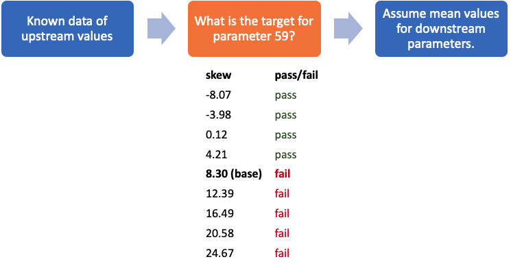
The model can be used by station engineers to decide what parameter to target based on 1.) what has already happened and 2.) assuming that downstream parameters will be their mean values. This is a reasonable assumption since the mean value is usually equal or close to the target values. In the above example case, a lot is at the station controlling parameter 59.
The lot ended up getting a value of 8.30 and failed. What if engineers at this station used the model to target a different value? What value should they target? The model suggests that the parameter should be 4.21 or less for the lot to have a good chance of passing. It is important to note that parameter control may not be perfect. For example, if 4.21 is the target, then the final result may be 3 or 5. In this case, engineers might want to target something lower to ensure being below 4.21.
Alternative Traditional Method
This is an alternative to the traditional method of targetting a population-wide control value and trying to get within the limits set by statistics of a distribution of lots. This method considers the specific history of this one lot.
What if parameter 59 ended up being 5.0? This is a marginal value and it is unclear whether the lot will pass or fail. This process can then be repeated in the subsequent stations where engineers can decide whether the lot can be saved if the required parameters to pass are achievable, or whether the lot should be scrapped early.
Using K-means Clustering to improve product variability
Intel, a leading U.S. semiconductor manufacturer is known for its philosphy of "copy exactly". This means that when a process in transferred from a development factory to a high-volume factory, engineers are challenged to replicate the tools, materials, recipes and operations as best as closely as they can. This same discipline is then maintained for succeeding high-volume factories. The idea behind this is that the customer should not care what factory a specific product came from. All Intel Core i7's of the same generation should all perform the same.
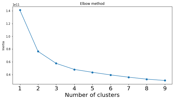
A scikit-learn K-means clustering model was used with clusters ranging from 1 to 9. Using the elbow method, it is shown that the optimal cluster number is between 2 and 3. A model with 2 clusters was used for further analysis.

Are the 2 clusters simply the "pass" cluster and the "fail" cluster? It turns out that it is not as shown in the table:
| Cluster | Passing rate | N |
| 0 | 92.8% | 1,245 |
| 1 | 93.5% | 322 |
There appears to be a majority cluster (cluster 0) and a minority cluster (cluster 1). This suggests that the process is yielding two different kinds of products.
The difference between 2 clusters
What is the difference between the 2 clusters? Normally, finding a difference would involve the following steps:
- Run a t-test or Analysis of Variance of all the parameters grouping by cluster.
- Get the p-value of each test. Conventially, p-values greater that 0.05 are said to be inconclusive.
- Rank the tests with increasing p-value. The tests with the lowest p-values are the biggest differences.
In this case, however, there is a big difference in population size (1,245 vs 322). SciPy suggests using the Kruskal test instead of ANOVA or t-test. The result of this process is 100 parameters with p-values <0.05.

The top suspect is parameter 162. Below is a boxplot of this parameter.

There is clearly a difference in this parameter between the clusters. A factory manager would prioritize scrutinizing this parameter with the goal of trying to eliminate this difference. Once this parameter is resolved or deemed untunable, then the factory manager can just go down the list.
Data Science Conclusion
To reiterate, the three ideas explored are:
- Accelerating inspection and failure feedback.
- Improving yield with better station-level decisions.
- Reducing product variability.
The methods proposed here cannot replace traditional operations done in semiconductor manfacturing. Traditional process control methods that have been refined over years will enable a player to compete in the semiconductor market. However, the novel methods proposed here can separate the good players from those that win the market.

