Price, Machine learning Housing Sale Price Prediction
The skills I demoed here can be learned through taking Data Science with Machine Learning bootcamp with NYC Data Science Academy.
Introduction
The purpose of this project is to build a model to accurately predict the sale price of the house. The dataset from Kaggle House Price Prediction Competition uses the Ames Housing dataset, compiled by Dean De Cock for data science education. With 79 explanatory variables that describe (almost) every aspect of residential homes in Ames, Iowa, this competition challenges students to predict the final price of each home.
My primary goals of this project are to achieve:
- Exploratory Data Analysis
- Data Cleaning
- Creative feature engineering
- Advanced regression models applied to the training data to accurately predict the sales price on the test data set
The Data Set:
The training set contains 1460 rows and, 81 columns, with 80 as features and one as target (the SalePrice). The test set contains 1459 rows and 80 columns.
There are 19 variables in the training data set which have missing entries. The magnitude of the missingness is shown in Figure 1. Test data set has 33 variables with missing entries, the distribution is similar to the training set.
Figure 1
In this analysis, I am focusing on the distribution of the target data and the relationship between the features and the price. Figure 2 shows the histogram of the SalePrice, our target variable. It is not normally distributed, but skewed to the right side. This needs to be rescale in order to have an accurate prediction with any ML model.
Figure 2 SalePrice Distribution
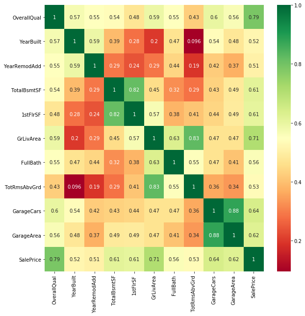
A heatmap in Figure 3 shows that the SalePrice are highly correlated with OverallQual, GrLivArea. This is very positive for developing an accurate model.
Figure 3 heatmap of SalePrice with other numerical variables
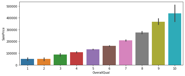
To dive deeper into the analysis, I plotted a couple of charts, Figure 4 and Figure 5. As Figure 4 shows, there seems to be a few outliers that need to be addressed. The relationship between OverallQual and SalePrice is a confirmation of their positive correlation characteristics.
Figure 4 Scatter Plot of SalePrice vs GrLivArea
Figure 5 Bar Plot of SalePrice vs OverallQual
Data Processing
Missingness Imputation
Most of the missing entries are due to the house lacking a feature: for example, garage, basement, pool, fence, alley. I can safely replace them with 0 if they have a numerical value, or none if they have categorical value. Other variables such as LotFrontage, masVnr, I will fill it with the neighboring median value.
Skewness
To address the skewness that some of the variables presented, I need to apply some form of transformation to de-skew them so that they will have a nice-looking normal distribution. Both log transform and boxcox from transform works well, and I choose to use the latter method.
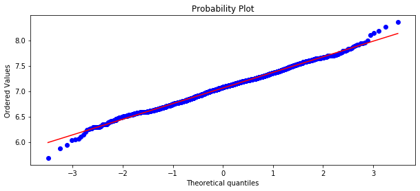
Figure 6 and Figure 7 shows the before transform and after transform of GrLivArea Probability Plot. We can see before the transform, the probability plot was a curving shape for GrLivArea, but after the conversion, it changed to a close linear shape.
Figure 6 Probability Plot Before transform of GrLivArea
Figure 7 Probability Plot of GrLivArea after boxcox Transform
I performed a log transformation on SalePrice. The outcome histogram shows it is close to a normal distribution.
Figure 8 Sale Price Distribution after Log Transform
Outliers
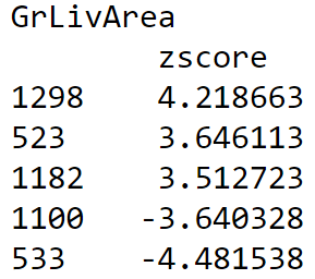
Outliers have a great impact on the models, it can skew the results of the prediction and so diminish its accuracy.. To address the issue, I use zscore function from scipy.stats to rank all entries from the numerical variables that have high correlations to SalePrice, i.e. GrLivArea, OverallQual, and filtered data points with high absolute zscores (>3.5), this process identified 4 outliers as shown in the next table.
I made my analysis on two groups, the first group with only two outliers from the largest of the ‘+’ and ‘-’ ends of the zscore list, (1298, 533). The second group has all the four outliers (1298, 523, 1100, 533).
Feature Engineering
1. Drop Features
Street, Utilities, ID are mostly irrelalivant to sale price, so it is safe to drop them from the data set. PoolQC has too much missingness, so it is safe to drop it as well.
2. Convert to Categorical Features
It would be better to have some of the numerical features in the original dataset in the categorical group, so the model can more easily spot them. If they stay in the numerical group, they will most likely be buried to the bottom. The following list are the conversions from numerical to categorical.
- 'KitchenAbvGr',
- 'TotRmsAbvGrd',
- 'BedroomAbvGr',
- 'GarageCars',
- 'HalfBath',
- 'BsmtHalfBath',
- 'FullBath',
- 'BsmtFullBath',
- 'Fireplaces'
After the conversion, the final data set has 49 categorical and 27 numerical features
3. New or Combine Features
I implemented a feature_engineering function to create new features by combining all the floor space features into one single feature TotalSF, Combining all the bath room features into one single feature TotalBath, add a few new features such as HaveFirePlace, HaveSecondFloor, etc.
4. Dummify Categorical Features
Categorical data needs to be converted numerical data by pandas get_dummies before I can use it to train any linear regression model. After the conversion, the dataset’s categorical features expanded from 49 to 309. But I used the drop-most technique to remove 49 entries from the categorical variables, this generated a training dataset (1458, 287) for two outliers group, (1456, 287) for 4 outliers group.
Modeling
Ridge Regression
Lasso Regression
ElasticNet Regression
Linear Regression Models include Ridge, Lasso, ElasticNet regression. Data for these models need to be prepared with dummyfication for the categorical variables. Then the training data was split into 80%:20% training test set. 80% used for training the models, 20% for validating the models.
The hyper-parameter for the linear models are simple; there is only one parameter for tuning in ridge or lasso models. ElasticNet has one extra parameter l1-ratio, so tuning takes more time than ridge and lasso.
The grid search function GridSearchCV from sklearn comes in handy, allowing me to specify the steps and range of the parameter, and set the number of folds to 5. That means the grid search function will split the 80% training data further to 5 parts, 4 parts for training, and 1 part for validation. It then uses the whole 80% training data to refit the model. This final model will be used for validation check.
Support vector Machine
Random Forest
Gradient Boosting
XGBoost
These models are non-linear models, and do not require dummification preparation for the training data. But the categorical data (usually a string type) need to be label encoded with sklearn LableEncoder. The training data will then went through the same process, split into 80%:20% training test sets. These models have a lot more hyper parameters, and their tuning is more complicated.
I grouped the parameters into 2 - 4 parts, with each part having 1-3 parameters. I tuned one group at a time, starting with fewer or coarser steps and a larger range, then narrower range and finer steps. If the parameters are sitting at the range boundary, I would expand the range and re-run the search. Once all the parameters in one group were optimally selected, I then moved to the next group and repeated the same steps. This process is very tedious and time consuming.
Once all the parameters are tuned for each model, I then applied the 20% test dataset to the model to check for overfitting.
Blending Models
Using a weighted average of all the models above, I can create a blended model. The weights was tuned using a top 1% submission as a training set, the mean square error root as the loss function. Here is the snippet of the code
Results
Models are compared using the metrics of normalized mean square error (MSE). The following tables shows the normalized MSE on all the models in cases of 2, 4 outliers removed. We can see all models are benefiting from outlier removal. Case 2 (4 outliers removal) definitely has much better performance than Case 1 (2 outliers removal).
Linear models are more robust than non-linear models, they are constantly producing better results. Fancy feature engineering like creating new or combining features may not be necessary and it did not make a big change to the model.
Case 1: MSE with two outliers removed
Case 2: MSE with 4 outliers removed
Case 3: MSE with 4 outliers removal +feature engineering.
Feature Importance
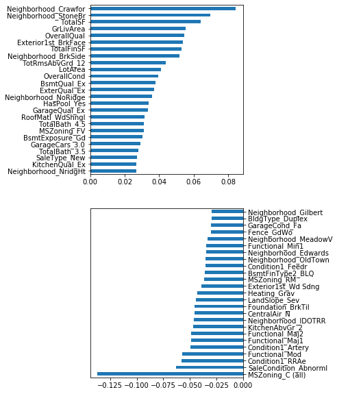
Figure 9 shows the top 20 positive/negative important coefficients from the ridge model. Figure 10 shows the important features extracted by the Gradient Boosting model. We can see that the living space, quality, and year built have positive impact on sale price of the houses. Bad zoning, no air conditioning, bad condition status have negative impact on the sale prices.
Figure 9 Linear Model Coefficients
Figure 10 Gradient Boosting Feature Importance
Based on the MSE value of all the models, I created a combined model using weighted factor. By tweaking the factor on each model, and compare the MSE with a top 1 submission in the kaggle competition, I was able to find an optimal combination for each outlier group. The following table shows my Kaggle scores. The best score I obtained is 0.11697, which put me within the top 16.2% of the participants in the competition.

Summary
Linear models such as Ridge, Lasso, ElasticNet are best for prediction, as they are simple to implement and easy to tune. But they are easily influenced by outliers.
Tree models such Random Forest, Gradient Boosting, and XGBoost are less prone to outliers, but they presented a challenge to overfitting.
A blended model from weighted average can minimize the above problems and produce a better result, but finding the right weights are challenging.
Data preprocessing such as boxcox transform, outlier removal, are critical in training an accurate model.
Future Work
Instead of using a top 1 submission for training my blend model for the parameters of the weighted average, I should investigate model stacking. I should be able to ensemble a set of models which uses weighted average to generate a blend model. I should be able to apply the same Grid Search to turn the weights using k-fold Cross Validation with training set.
The source code is in github


