Predictive Analytics - Allstate Claims Severity
Introduction
The Allstate claims severity challenge was a Kaggle competition that was open in 2016. The task at hand was to perform predictive analytics to find claim severity. A training dataset containing 116 categorical variables and 14 continuous variables was provided. Each row represented a claim. Along with the predictor variables, there was also the actual loss on that claim.
The training dataset contains 188,318 claim records. The prediction task was to find the loss for each of the 126546 claims in the test data set.
The scoring was done based on accuracy of submissions that were made on claim severity of a separate test file that was provided. This file did not have the loss column.
My Workflow
Training
- Load Train Data
- Data Visualization
- Data Preprocessing
- Model Selection
- Feature Selection
- Model Training
- Model Validation
- Execution of model on new data
- Ensembling of models
- Extreme Gradient Boosting
Prediction
- Load Test Data
- Data Preprocessing
- Model Execution on Test data
- Creation and submission of the prediction
Loading of data and visualizations
allstate=read.csv("./train.csv")hist(allstate$loss)
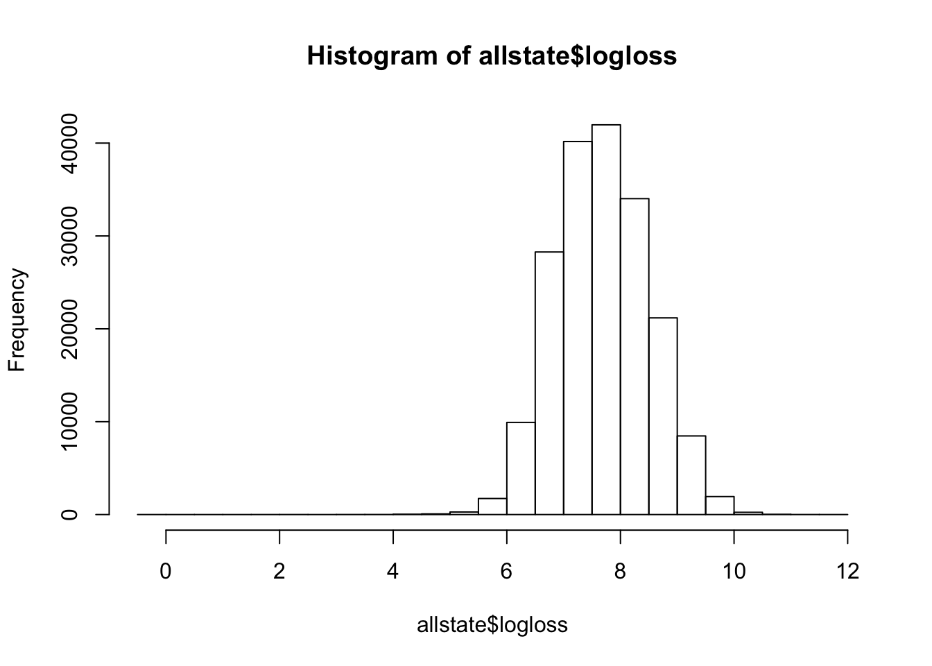
We see that the loss itself is heavily skewed to the left. This has an implication when it comes to model training. I found that by using logarithmic functions on top of loss, the distribution was made to be much more normalized and this helped in getting better predictions.
To further visualize all the fields, a for loop was used to create charts on each of the variables.
carvars = paste("cat", 1:116, sep="")
par(mfrow=c(29,4))
for( catvar in 1:11){
   catvar <- paste("cat", catvar, sep="")
   p <- ggplot(allstate, aes_string("logloss", fill=catvar)) + geom_histogram(binwidth = 1)
   print(p)
}
Loading the train data
Partitioning of the data
We are going to take 80% of the train data and use it for our model training. The remaining 20% of the data will be used to determine how well our model worked.
set.seed(1234)
# define an 80%/20% train/test split of the dataset
split=0.80
trainIndex <- createDataPartition(allstate$id, p=split, list=FALSE)
data_train <- allstate[ trainIndex,]
data_test <- allstate[-trainIndex,]
Feature Selection
To optimize our models, we will need to take a subset of the features available. I chose to run the rpart model on the entire dataset to come up with the fields that we need.
catfactors <- paste("cat", 1:116, sep="")
contfactors <-paste("cont", 1:14, sep="")
formula = reformulate(termlabels = c(catfactors,contfactors), response = 'logloss')
modelFit <- train( formula,data=allstate, method="rpart" )
varImp(modelFit)
cat80D 100.00
cat80B 99.75
cat12B 78.30
cat79D 75.14
cat79B 59.11
cat10B 18.35
cat1B 18.27
cat81D 16.09
cat81B 14.15
Execution of various models
The following models were tried and the best scores were obtained by the XgBoost model.
- Linear Regression
- Rpart
- Xgboost
catfactors <- c(“cat80”,“cat12”,“cat79”, “cat10”, “cat1”, “cat81”)
formula = reformulate(termlabels = c(catfactors,contfactors), response = ‘logloss’)
ControlParamteres <- trainControl(method = “cv”, number = 10, savePredictions = TRUE, classProbs = TRUE, verboseIter = TRUE )
parametersGrid <- expand.grid(nrounds=100, lambda=.5, alpha=.5, eta = 0.1 )
model.xgboost <- train(formula, data = data_train,method = “xgbLinear”, trControl = ControlParamteres, tuneGrid=parametersGrid)warnings() summary(model.xgboost)
Validating the model
# Validating our model
x_test <- data_test[c(catfactors,contfactors)]
y_test <- data_test[,"logloss"]
predictions <- predict(model.xgboost, x_test)
str(predictions)
head(y_test)
str(predictions)
hist(predictions)
#Computing RMSE and R2
caret::RMSE(pred = predictions, obs = y_test)
caret::R2(pred = predictions, obs = y_test)
Predictions on the test file
prediction.testFile=read.csv(“./test.csv”)
out_test <-testFile
id <-out_test$id
str(id)
logloss <- predict(model.xgboost, out_test)
loss <- exp(logloss)

head(loss)
hist(loss)
Creating the submission file
out_file=cbind(id,loss)
head(out_file)
options(scipen=999) # Removing the exponential format
write.csv(file=“./submit.csv”,out_file,row.names = FALSE)
Challenges faced
The data is highly anonymized and this prevented any kind of feature engineering on top of the data provided. Using Domain knowledge to fine tune our models was almost impossible.
The large set of features slowed down the models by a huge extend. In the interest of creating a model that is of practical use, I had to select the features to use. The lack of domain information led to possibility of errors while eliminating features for training.
Results
I was able to learn how to apply various models. Caret as a package makes adoption of various models a breeze. I was also able to start using RMarkdown as a documenting tool while developing models.


