Studying Data to Predic Housing Prices in Ames, Iowa
The skills the author demoed here can be learned through taking Data Science with Machine Learning bootcamp with NYC Data Science Academy.
Predicting Housing Prices in Ames, Iowa
By Ariani Herrera, Erin Dugan, John Nie, Won Kang
This Kaggle Competition offered a comprehensive dataset of nearly 4000 home sales in Ames, Iowa between 2006 and 2010 with the various features influencing the sale prices. Our motivation was to explore and analyze the housing data to find the key features that influenced the sales price and then develop a machine learning algorithm to predict the prices.
Exploratory Data Analysis and Data Transformation
Upon observing the data, our team wanted to create a systematic method to understand the variables before building any sort of model. We sorted through a sample of the data set which included 79 explanatory variables and the corresponding sale price for each home. Our team explored the different data types within the data, which were divided into 38 numerical features and 43 categorical features.
To predict the housing prices, our team explored the variables to evaluate the key features that affect housing prices in Ames, Iowa. We then wanted to understand redundancies, collinearity, and the relationships between different variables.
Correlations
We began our Exploratory Data Analysis by examining correlation between the features. The heat map below shows the correlation between all the features in the data set. The darker or lighter the color (correlation is either close to 1 or -1), the stronger the relationship between variables. From this graph, we are able to see which features had the greatest influence on the Sale Price and note the correlation amongst the features. If there is multicollinearity, or a strong correlation between features in the model, it can contribute to errors in the model. For example, both GarageYrBlt and YearBuilt were highly correlated, so only YearBuilt was used in the prediction model.
Our team also wanted to remove information that did not seem relevant or useful. If a variable was missing more than 50% of its data, we removed those columns from our dataset. The graph below is a visual representation of the missing data.
For other variables having a significant portion of missing data, we decided to make educated assumptions to impute the missing data, such as with Lot Frontage. After some research, our team felt it was fair to assume that we could impute the missing Lot Frontage value with the average frontage for that particular neighborhood, as most in a given neighborhood do not deviate significantly. For other features with missing values, we imputed the missing data with zero or None, depending on the feature.
Excluding the Outliers
Generally speaking, outliers are observations that appear to deviate outside the overall pattern. Also, extreme outliers could dramatically impact the results of a prediction model. We conservatively removed two outliers, which were homes with sale prices over $300,000 and had less than 4,000 square feet of living area. After the outliers were removed, the graphs depicted a more linear relationship between sale price and square footage.
There were certain numeric variables that actually described categorical features. In the graph below we illustrate this was the case with the month sold. While sales varied by month, there was no numerical pattern represented by the month of the sale.
Some categorical variables showed ordinal features. Kitchen Quality, shown below, is an example of where an excellent kitchen increased the value of a house. Our team ranked the different kitchen qualities for our model to prioritize the kitchen quality if it is excellent (Ex) over if the kitchen quality was good (Gd), typical/average (TA), or fair (Fa).
Skewed distributions can decrease the accuracy of a model’s predictions because it could reduce the impact of low frequency values which could be equally significant when represented by normally distributed data. As shown in the graphs below, we used a log transformation to normalize the Sales Price. Other skewed features, such as Lot Area, were also adjusted in the same manner.
Machine Learning Model Development
After cleaning and transforming our data, we explored various machine learning algorithms to predict sales prices. To investigate benefits of dimension reduction and look for strong patterns in the dataset, we also evaluated the models with and without Principal Component Analysis. The various machine learning algorithms were optimized with a parameter grid search and used K-Fold cross validation to prevent overfitting. The two paths used in developing our models are shown below.
Our team built a comprehensive and robust model that explored Linear Regression, Lasso, Ridge, Elastic Net, Kernel Ridge, and Random Forest regression models and used a grid search with K-fold cross validation to ensure we had optimal tuning parameters.
We tested these models with and without Principal Component Analysis (PCA). After cleaning our data, performing EDA, and creating dummy variables for the categorical features, there were over 318 features in the model. 85 Principal Components accounted for 90% of the variance in our data. PCA allowed for us to reduce variation and illustrate strong patterns.
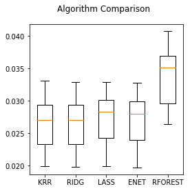
The chart below shows our results after completing Principal Component Analysis for the Kernel Ridge, Lasso, Random Forest and Elastic Net models. With PCA, the Kernel Ridge, Lasso and Elastic Net models performed the best in predicting housing prices with a Root-Mean Square Error of approximately 0.026 - 0.027.
Unfortunately for our models, PCA has its limitations since it relies on linear assumptions. Although PCA does a great job with data that is linearly correlated, PCA might not capture the full picture if there are nonlinearities.
Models Without PCA
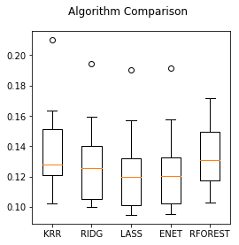
Our team also ran the models without PCA and as depicted in the graph below. These results indicate models using Ridge, Lasso, ElasticNet, and Random Forest perform better without PCA best in predicting housing prices with a Root-Mean Square Error of approximately 0.024 - 0.029.
Finally, once we optimized our models based on the training data, we ran the Kaggle test set through the algorithms to predict the sale price. Overall, the ridge model provided the most accurate predictions.
Conclusion
From this project, we gained several key insights and ideas for improving the model in the future. While implementing PCA in the model did not always provide improved predictions, it may have improved results if we are able to identify any nonlinear relationships within our data set. We believe the grid search to optimize the input parameters of each model improved the accuracy and could be further improved with additional tuning among a broader range of parameters.
Additional regression models could also be implemented into the algorithm to optimize results as well as model stacking or ensembling techniques to incorporate several models into the prediction. Other considerations may include investigating other data that could influence the prices, such as how long the home was on the market and whether it has a desirable layout. It would also be interesting to see how these models perform based on home sales outside the dataset, for years after 2010.


