Data Analysis and Predictions: The Estate Saints
The skills I demoed here can be learned through taking Data Science with Machine Learning bootcamp with NYC Data Science Academy.

Objective:
Predicting the value for a house can be a useful tool for consumers and real estate practitioners. The quality of a house and its surrounding features potentially make or break a buyer's decision and determine the overall price. A buyer is always thinking the same thing, “Am I getting the best bang for my buck?” It’s a no brainer, you want to make sure you are getting your full money’s worth, and why shouldn’t you?
The Data:
The Ames, Iowa housing data set was obtained on the Kaggle website, which contained 79 featured aspects of a residential property from 2006-2010. Some of those features included location of the property, property size, overall condition, roof styles, and year of the house. This dataset included in depth descriptions of the features collected and how to interpret each individual observation.
EDA:
To understand our collected data further, we started by identifying columns with high missing data. We wanted to see if there were features that did not seem important or would add value; these columns would be considered to drop. We used basic visualizations like a correlation matrix to understand which columns had high collinearity with each other such as garage area and the amount of cars a garage holds. We would need to reduce this to be able to have accurate results for our models.

For further analysis, we used some scatter plots and line graphs to see how certain features interacted with each other to try and understand trends that would affect our overall goal to predict the value a house should be priced. Our end goal is to reduce the number of features that are highly similar with other features or will not contribute highly towards our model to reduce the complexity and highlight the most important features.

Lasso Regression Model:
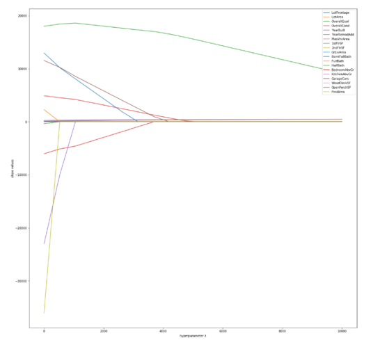
Through our initial EDA, we saw our data had a relatively linear trend. We wanted to use a linear model so we chose a Lasso Regression model to predict housing pricing and help reduce multicollinearity through classification. The lasso regression model introduces a penalty to regularize the model; this helps lower the error of the model at the cost of some accuracy. Through hyperparameter tuning, the lasso model can actually reduce coefficients to zero which is why it can be used for classification.

We split our model into a 70/30 training set and test set to score and record error when trying to predict house pricing. Our model showed pretty high accuracy, but also higher error than anticipated showing it was overfitting our prediction. By dropping features that had high multicollinearity shown by our classification, we were able to decrease our error and maintain high accuracy.
| Train R^2 | Test R^2 | Mean Squared Error |
| 0.8861 | 0.8954 | 0.02530 |
Figure 3. Table of accuracy and error for Lasso Regression Model
The client is everything to us, we wanted to test other models to see if we can outperform our first attempt. We chose an elastic net model to compare to our lasso model. The elastic net combines the penalty terms from a lasso regression model with one from a ridge regression model as well. Each regression can be given a weight of importance through hyperparameter tuning. Our Elastic Net model showed similar results to the lasso, but overall had a higher error and lower accuracy for the test data proving our lasso regression provided the best results in predicting house pricing.
| Train R^2 | Test R^2 | Mean Squared Error |
| 0.8970 | 0.8893 | 0.02107 |
Figure 4. Table of accuracy and error for Elastic Net Model
OlS Regression Model:
Backward Elimination Wrapper Method
We used a wrapper method to perform the evaluation criteria when selecting which features to keep in the model. We fed all 79 features to the selected machine learning algorithm and based on the model performance we added/removed the features that were highly correlated to the sale price. This helped us to identify which features were of importance to our idea and which features we should keep.
K- Fold Validation – 5 Splits
We then evaluate our models performance based on an error metric to determine the accuracy of the model by using the K-Fold Validation – 5 Splits.
Cross-validation scores: [0.88838404, 0.7851076, 0.84647181, 0.83752568, 0.69006605]
Random Forest Model:
We wanted to test a nonlinear function that could also perform classification to compare to our previous models; we chose a random forest as it meets both criteria. The random forest is an ensemble method that implements multiple decision trees using random sampling. Each tree outputs a class prediction,the class that has the most votes becomes the prediction for the model. The random forest uses these best results from uncorrelated trees and combines them together. Through this ensemble, all of the weak models come together to create one strong and stable model.
| Train R^2 | Test R^2 | Root Mean Squared Error | Mean Squared Error | Mean Error |
| 0.9666 | 0.8757 | 29225.4910 | 854129322.44 | 18619.36 |
Figure X. Table of accuracy and error for random forest model
Our random forest model had high accuracy, especially with our training dataset. We were able to identify some of the key features that drive someone to buy a home. Overall quality, overall condition and masonry veneer were among the most important features found with the random forest.
Conclusion:
Our models determined which features add the most value to a house compared to others. This can help sellers and contractors increase house value further by fixing up or improving features identified by our model that would increase the price. Our models help increase real estate value for the consumer and the supplier.

