NFL Analysis: Spend by Position and the Impact on Team Performance
The skills the authors demonstrated here can be learned through taking Data Science with Machine Learning bootcamp with NYC Data Science Academy.
The code for this project can be found on my GitHub page.
Introduction
As the 2018-2019 National Football League season comes to a conclusion tonight in Atlanta, all 32 teams will be gearing up for the offseason. But how should they allocate their money for next season and beyond? This is a fundamental question that each team's decision-makers must toggle with. While I would have liked to scrape and analyze more years of data, complete historical NFL salary cap data is difficult to obtain.
Objective
The objective of this data analysis is to examine positional spending and win percentage across all 32 teams in the NFL from 2013-2018.
The NFL Salary cap is broken into many sub-components. For the purpose of this analysis, I included all team spend with the exception of “Dead Cap”. Since I wanted to measure the impact of actively contributing players (and “Dead Cap” is dollars spent on players who are no longer on the roster), I felt it was best to exclude these figures in my study.
Web Scraping
In order to compile the data for analysis, I used Scrapy to extract the relevant data from both Spotrac.com/NFL for Salary Cap data and pro-football-reference.com for Win/Loss data.
To scrape Spotrac.com, I built a web scraper to first loop through every team’s positional spending page, then loop through every year from 2013-2018.
Below are screen shots of both the Spotrac.com/NFL homepage and an example of a team page.


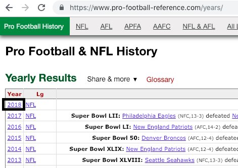
For pro-football-reference.com, I built a web scraper to loop through the years 2013-2018 and scrape standings data for team Win %, Points For and Points Against statistics.


Data Cleaning
Once I extracted the data into two separate CSV files, I used Python to clean the data in preparation for analysis. The main steps I took to do so were:
- Merging CSV files (grouped by Year and Team Name) into one Data Frame
- Year and Team Name were the two common fields in both data sets I was joining
- Creating additional columns
- Since the data I retrieved was in absolute dollars spent by positional group/team/year, I created a ‘Spend %’ column to apply to each row of data
- I also added some custom fields for analysis, aggregating positional group spend percentages for further analysis
- Creating sub Data Frames for each year of data

Data Analysis
Positional Allocation % by Year
The first piece of information I wanted to analyze was allocation trends by position over the years. In the below chart, I broke down spend % by each positional group.
From left to right, the positional groups analyzed are Offensive Line, Quarterback, Running Back, Wide Receiver, Tight End, Defensive Line, Linebacker, Defensive Back and Special Teams.

As you can see (and much to my surprise), there has been very little variance in leaguewide positional allocation percentages over the past 6 years!
Positional Allocation % vs. Win %
Over the past 6 years, the leagues positional allocation percentages have been extremely constant. But how did spending by position attribute to wins and losses?
I created correlation matrices to assess this relationship:


As you can see (and much to my surprise, again!), there was no statistically significant correlation between % of team spend on any of these positional groups and/or stacks vs. win %.
The below scatter plots further illustrate this lack of a correlation:


Ideas for Future Development
I plan to continuously evolve and expand this analysis. The opportunities are endless, but below are a few ways I’d like to do so:
- Scrape team statistics and run regression analyses on team stat metrics, positional spend and win %
- Analyze team specific scenarios (i.e. outliers- The best and worst teams, as well as teams with large YoY variances in win %)
Final Thoughts
As the NFL has evolved over the years by way of rule changes, strategy adjustments and the like, I expected to see significant variances in positional spend % by year. That clearly has not been the case.
Why have we been so constant and how can teams gain an edge by allocating resources differently than the herd? I look forward to continuing to develop this analysis and uncovering more insights on the NFL allocation puzzle.
Enjoy the Super Bowl everyone!


