A neural network trained in anomaly detection
It is well known that neural networks are one of the most sophisticated regression and classification models, able to model complex non-linear relationships and surpassing the a priori need for feature engineering. This is because selection is encoded in the hidden layers: each hidden node 'selects' one (or more) anonymous features and assigns it a weight before activating the next layer of neurons.Each subsequent layer of the network 'learns' increasingly more complex (and invariant) combinations of features. This is repeated for each feature and throughout each hidden layer until an output activation is reached. Many of the modern deep learning techniques are scaleable, applicable to a wide range of regression problems, and incredibly elegant.
This code was written for the Kaggle Santander competition, but provides a robust and general approach towards K-classification problems with highly imbalanced classes. The training data set consists of over 300 anonymized features and nearly 80,000 observations, most of it sparse, bugged (-999,999 in a row consisting of otherwise small positive integers) and with a target column of 1 representing unsatisfied customers, and 0 representing satisfied customers. Many popular and competitive approaches include XGBoost for gradient boosting as well as naive Bayesian classification. In this exposition we present two alternative methods in gradient boosting and deep learning networks, where we fine tune the methods to detect the minority class of 1's from 0's (1's comprise less than 4% of the overall target, and 0's comprise the rest.)
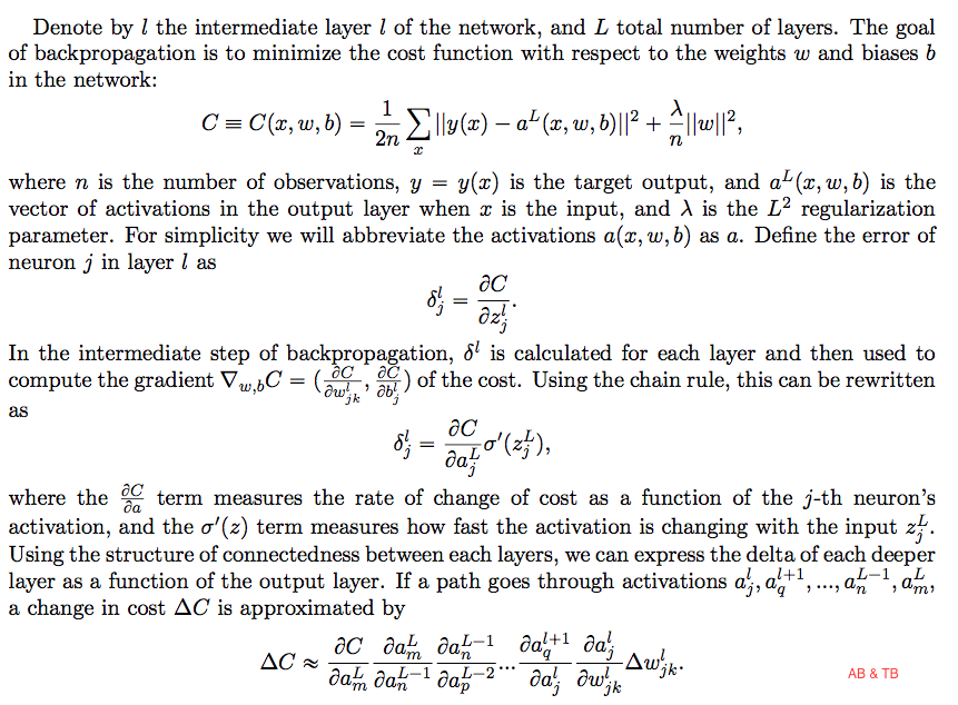
For a full explanation of the mathematical theory where most of this summary derives from we refer to, and thank, Michael Nielsen and his Neural Networks and Deep Learning book. Below is a summary of the backpropagation and stochastic gradient descent algorithm where we introduce our notation. We will state the calculus equalities without proof.

The backpropagation algorithm and stochastic gradient descent
The backpropagation algorithm can be coded as follows. For each input x, we use a traditional feedforward network to compute the weighted input z for each layer. We compute the output error delta for L and then backpropagate this for l = L-1,...2. We then compute each component of nabla C, for every component of the input x.
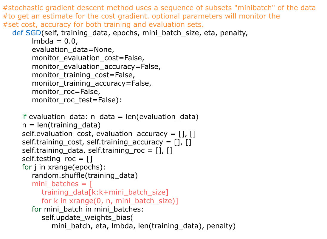
The heuristic sense of delta as the 'error' term is visible in the stochastic gradient descent algorithm. Rather than using all observations to compute the gradient nabla C, we take a random sample of size m called "mini-batch" and approximate
in order to speed up each computation. For each randomly chosen mini-batch of training inputs, and for each l = L, L-1, L-2,....2, we update each weight and bias with the rule:
Note the sum is over all training inputs in the minibatch. Alternatively, if one uses an unregularized cost function, the second update rule is replaced with
Here eta is called the learning rate. It must be small enough that the Taylor expansion of C is still valid, and small enough that we do not overshoot the cost function minimum, while fast enough that the network learns to minimize the cost.
We are ready to code the network class. A preliminary step is to clean the data so we throw away useless information, debug faulty variables and remove zero variance features. (These can in principle be weeded out by the neural network, but for the purposes of clearing space we delete as many columns as possible.) For maximal efficiency we delete low feature importance features after fitting a random forest model to the data, and then finally normalizing both the training and the test set.
Cleaning data, removing constant and identical features, and using k-nearest neighbours to debug 'var3':
An anisotropic cost function
What is the most significant problem with our target set? The majority class makes up 96% of the data. This means that our neural network, being smart, will learn to guess zeros uniformly in order to achieve a 96% accuracy. This is a default base score. The reason for this is that the quadratic cost function we are using is non-discriminatory in classes:
We need a better descriptor of our cost hypersurface on which the network can learn. Rather than give equal weighting to the 1 class and the 0 class, we force our network to learn more aggressively on the 1's by implementing a penalty for misclassification of 1s. We can simply amend this function to
This still satisfies the fundamentals of a cost function, and is still quadratic in the |a-y| terms! The gradient of the cost will only change by a linear factor depending on the penalty: we have now delta = penalty(y_i)||a-y|sigmoid'(z)x_i. We now have a dictionary of penalties with which to tune the network. (Note this is generalizeable to a classification problem with multiple classes.) These act as multipliers in the delta function, the gradient of cost, and implicitly appear in each update of weights and biases. Intuitively, penalty(y = 1) should be much greater than penalty(y=0), forcing the network to care more about misclassified 1's than 0's. This is analogous to using a faster learning rate on the minority class when implementing a traditional gradient descent algorithm, but loses this interpretation when the gradient descent is stochastic: we do not know a priori what the distribution of 1's and 0's will be in the minibatch samples, so the penalties will become a weighted average of target-dependent learning rates. It is similar to the idea of a support vector machine with discriminatory class weights:
We now summarize the main brute force of the code below.
The cost & delta functions and main Network class
On regularization, neural saturation and the learning slowdown
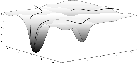
Several things happen when the network is trained. We want to avoid fluctuation of the weights between epochs. It is important to avoid the quandary illustrated above: the learner getting stuck in local minima of C(w,b). In order for maximal efficiency of gradient descent, it is important to understand what happens when randomly initializing weights generated by a normal distribution with mean zero and variance 1. It is quite likely that |z| will be large, which means that sigmoid(z) will very nearly hit one. This saturates the neuron and turns it into a pseudo perceptron, which means small updates in the weights will make negligible changes in the activation of proceeding neurons. This in turn will have a negligible effect on the activation of the next hidden neuron and so forth, resulting in a cost "stuck" in a local minimum. Gradient descent won't save us, and the network learns very slowly. We remedy this by using Gaussians with mean zero and variance 1/n.
Secondly, the weight initialization is random and sometimes the network gets stuck on a higher-cost surface when we have an unlucky combination of initial weights. We recover from this by giving our network 'memory', or the ability to store the best possible weights and biases over all the weights and biases that it has so far seen.
The last phenomenon that happens to us is a slowdown when lambda is too small. Because neural networks have many more weights than inputs, overfitting is a common problem. Over time, the magnitude of weights tends to increase after each epoch. The effect of lambda is to force the network to prefer to learn small weights, all other things equal, and to compromise between fallaciously minimizing the cost function and shrinking the weights. We notice that over several hundred epochs of training, the norms of the weight vectors grow in magnitude. This causes dC/dw to get stuck in the same direction, since changes from the SGD algorithm make negligible modifications to delta when ||w||^2 is very large. We again get stuck in a local minimum, unable to traverse the entire cost surface, and learn very slowly.
Remark: One can prove the four fundamental backprop equations for any activation function (not just the sigmoid) and could potentially design any activation function so long as it satisfied (4). To avoid the learning slowdown that can manifest in training, we could choose a sigmoid function so that sigmoid prime is always positive and bounded away from zero.
Making the network learn faster without changing the learning rate
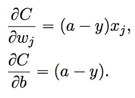
Can we speed up learning without modifying eta? It happens that on several epochs the network stops learning, or learns very slowly. The reason for this is because of the appearance of the derivative of sigmoid in the gradient of the cost:
The latter sigmoid'(z) term means that when the neuron's output is close to 1, the s-shaped sigmoid curve gets flat, so its derivative is close to 0, and updating the weights and bias proceeds very slowly. Hence the size of the error term a-y does not affect the rate of learning. What we seek is a cost function such that
which captures the moral of faster learning on greater initial error: the gradient of the cost should be steepest when a-y is large. Absence of the sigmoid'(z) term also relieves the issue of a learning rate dependent on the shape of the activation function, which exacerbates the slowdown caused by neural saturation. We can formalize the problem by solving the equations
This motivates the cost entropy function
Much like the anisotropic quadratic cost, we can implement a penalty rate depending on whether or not y outputs a 1 or 0 by adding the multiplier
The second issue is the shape of the sigmoid function.The problem with the usual sigmoid activation function is that the output of each neuron is bounded on the interval [0,1]. This induces a systematic bias for neurons beyond the first layer, but we want to avoid inputs to layers which have non-zero mean and avoid saturation. This can easily be done on the first hidden layer by rescaling the data, but we have no way of controlling this on remaining hidden and output layers of the network.
The key to solve this problem is to use an antisymmetric activation function, such as the hyperbolic tangent, which can be expressed as 2*sigmoid(2z)-1. It shifts the output interval to [-1,1]. Thus we rescale the activation function from the blue curve to the red:
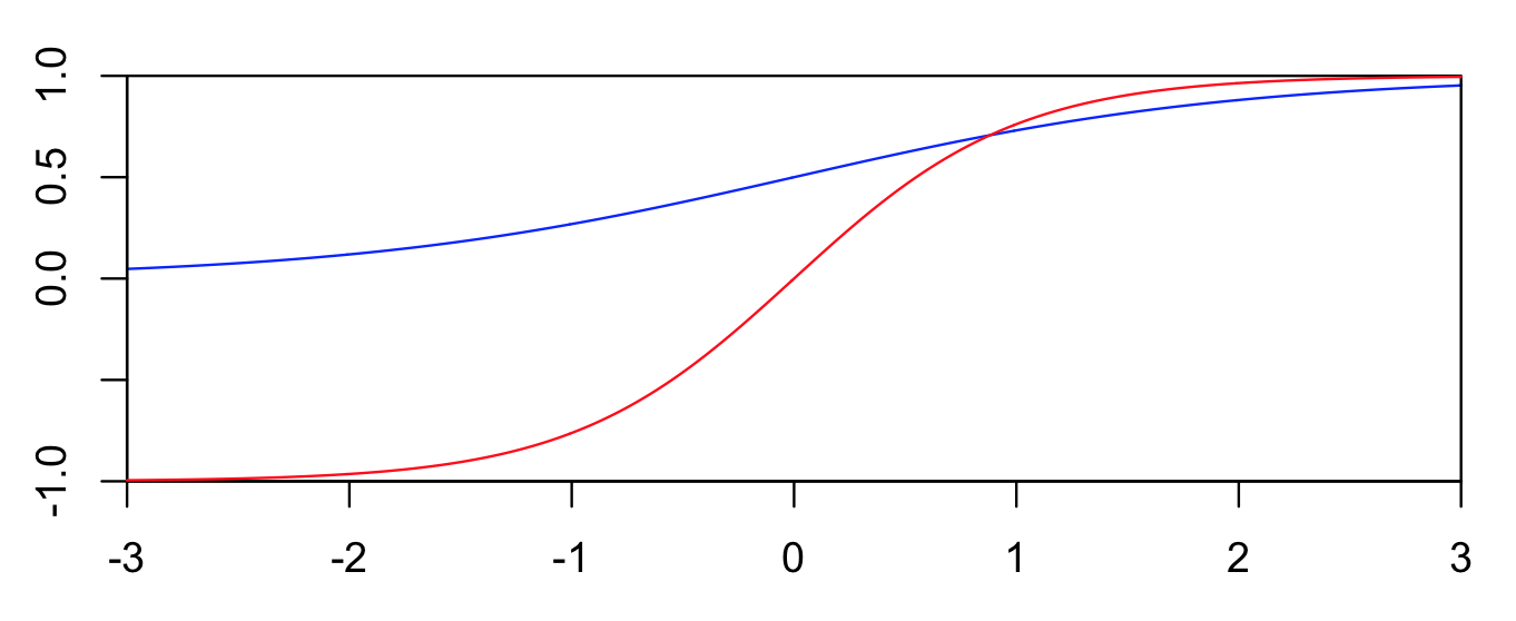
With this choice, the output of every neuron is allowed to take either positive or negative values in the larger interval, which means its mean is likely to be zero, and the hidden neurons are less likely to saturate. For large hidden network topologies, backpropagation algorithms and antisymmetric activation functions produce quicker convergence than the standard process.
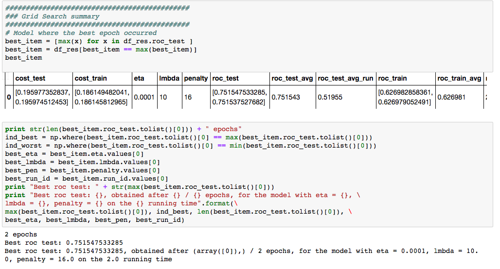
We end with a description of our grid search. Because of the numerous tuneable parameters, this quickly encompasses a search through over thousands models. For the sake of computational feasibility, we often had to restrain ourselves to only a few hundred different models. To select the models within the grid, we first split the training set into a training part to fit the model and a testing part to test our results and prevent us from possible overfit. Both parts are samples from the training set, and we may choose to either sift through the entire data, or to select only small samples. The dataset being large (about 76,000 observations), choosing a small sample (a different one every time we try a new model) will speed up the search but is likely to poorly represent the full dataset, even more so as the proportion of 1's is so small. We therefore try to find a compromise and in the code below choose to train and test over samples that contain 10% of the observations. In order to find the most appropriate combination of parameters, we sift through different arrays that represent the penalty (Pen), the regularisation (Lmbda), the learning rate (Eta), and the number of times we wish to run the same model (Run_count, so we make sure a good result for a particular model is not only due to a lucky hand in randomly picking the initial weights). In addition to these parameters, we also offer to modify the Network's Topology by introducing a nested list (Config) of which each element is the list of the numbers of neurons for every hidden layer. At each step of the loop, we save our results in a DataFrame names df_res to keep track of every model's performance.
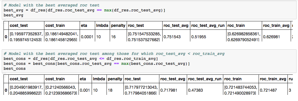
On the pictures above, we show a result from a grid search. We first look at the model that realised the best ROC AUC test score. In order to find the more stable model, we then average over the different epochs and over the different times we are running the same model.
A gradient boosting machine
A much easier, and yet powerful method to tackle a classification problem, is to use XGBoost. It is a boosting method that relies on building successive trees for which the error of every new tree depends on the errors of the previous ones. This way we ensure that every new tree is as low correlated to the others as possible and actually do bring new information to the model. Unlike neural networks, tree based methods require the data's features to be cleaned and organised before being fed to the model. In the code below, we first remove the similar features, that is the columns with similar observations, and then use a Random Forest as toy model to identify the most useful features. A closer look at the outliers then shows that some of those for which a feature attains its maximum seem to be relevant in deciding wether the target variable should be either 0 or 1. Here we simply focus on these particular maximum outliers by removing them from the feature where they appear, only to add them again on a new column for the same observation. We thus add two new columns, one for which the maximum outliers are classified as target 1, and another for which they are classified as target 0. In order to tune the parameters and find the best model, this time we use an automated Cross-Validation function from the sklearn package. After our first attempt , we obtain a ROC AUC training score of about 0.83.


