House Prices Prediction Using Machine Learning
Introduction
The goal of this project was to utilize supervised machine learning techniques to predict the price of house located in Ames, Iowa. The dataset was provided by Kaggle, an online community of data scientists and machine learners, owned by Google.
This dataset provides 1,460 observations and 80 features, including multiple aspects of the house that may or may not help predict the fluctuation of the house prices.
The strategic approach our team adopted was to derive meaning from the dataset through numerical and visual exploratory data analysis, drop statistically irrelevant features and features with high multicollinearity, impute missing values, create new features, and then apply different supervised machine-learning algorithms to predict the housing sales prices.
EDA
As you can see below, transforming the data was important due to the skewness of the overall data.

Exhibit 1. Skewness of Features
The first transformation we performed was on the sale price. You can see that before the log transformation, the data was heavily right-skewed. After the log transformation, though, the sales price achieved an approximately normal distribution, and the skewness value dropped from 0.188 to 0.12

Exhibit 2. Density Plots of Target Variable Before & After Transformation
Dealing With Missing Values (NAs)
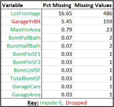
First, we dealt with features almost exclusively filled with NAs that had explicit meanings and did not represent missing observations. For instance, two features referred to pool quality and condition. However, only 7 houses had a pool while NAs in that column meant that there was no pool. In the same way, the NAs in the alley column meant that there was no alley access, NAs in the fence column meant that there was no fence, and the NAs in fireplace column meant there was no fireplace.

Exhibit 3. Missing Values in Features
When imputation wasn’t feasible due to lack of information, we dropped the feature. When imputation was feasible, we either replaced the NA with its actual meaning, or we imputed using mean, mode, or 0.
Outlier Removal
Another way to reduce the skewness is by removing outliers. This procedure is not an easy task and having domain knowledge is usually an advantage. One way to remove outliers is by deleting observations of features which are three or more standard deviations from the mean. However, in our case, this would remove hundreds of observations from the dataset. To avoid such a huge data loss, we created a scatter plot of sale price versus other features and decided to remove the four most apparent outliers.

Exhibit 4. Outliers in the Scatter Plot
Feature Engineering & Selection
Feature engineering is fundamental to the application of machine learning, so we individually analyzed features and discussed their relevance to this project.
For categorical data, we observed each features' relationship by comparing the mean and median sales prices of the different groups using ANOVA and boxplots respectively.

Exhibit 5. Boxplot of Overall Quality vs. Sale Price
For numerical data, in order to avoid high multicollinearity, we examined regression plots for each numerical feature against sale price and created correlation heat map for all numerical features.

Exhibit 6. Sample Scatter Plot and Heat Map
Based on our results from the previous steps, we decided to drop features irrelevant to the sales price as well as features with high correlation. For example, ground living area square feet was equal to the sum of first-floor square feet, second-floor square feet, and low quality finished square feet. Thus, we decided to drop the last three and only keep ground living area. We dropped a majority of the quality and condition columns because we assumed that “OverallCondition” and “OverallQuality” described all these other features.
We also replaced ordinal categorical features with corresponding integers. For instance, we encoded the lot shape feature as follows: A regular shape was assigned the value of 4, slightly irregular a 3, moderately irregular a 2, and irregular a 1.
Lastly, we added a new feature: "YrSinceRemod". This new feature equaled to year sold minus remodel date, thereby capturing the number of years since a house was either last remodeled or built. Moreover, instead of putting in all the bathroom features separately, we created a combination value named “Total bathrooms” that included basement full bathrooms, full bathrooms, basement half bathrooms, and half bathrooms.
Modeling
To find the best fit for our data, we decided to apply both linear and non-linear algorithms:

Exhibit 7. Modeling Workflow
Linear Regression (Ridge, Lasso, ElasticNet)
We decided to begin our modeling process linear models after normalizing the independent and dependent variables.
The first model out of the linear regressions we used was the multiple linear regression model. The root mean squared error (RMSE) for the multiple linear regression was 0.18. The reason the error was so high was most likely because this model has no penalization for the number of features used and therefore is prone to multicollinearity issues.
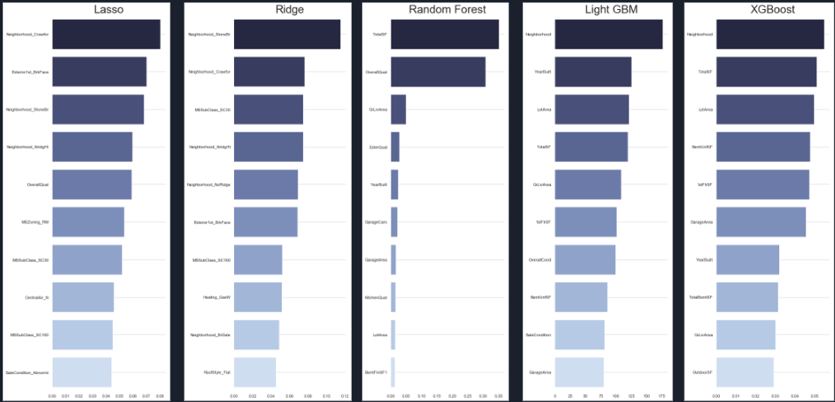
After that, we tried the penalized regression models: Lasso, Ridge, and ElasticNet. For each of the models, several neighborhood features received a significant importance in the feature importance output, suggesting that the neighborhood greatly impacts the sale price.

Exhibit 8. Feature Importance from Lasso
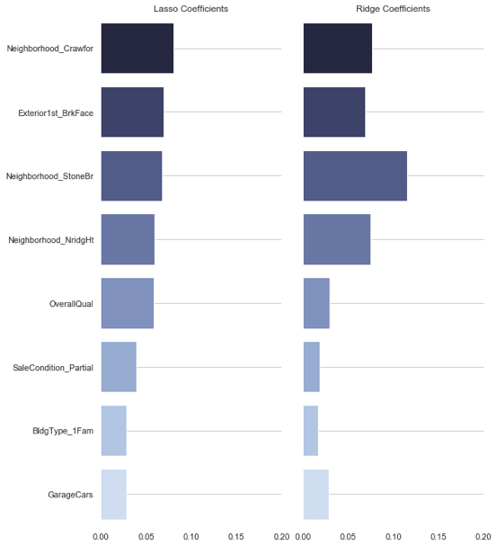
Out of all the regressions we implemented, lasso regression achieved the best RMSE, 0.124, probably due to actually dropping features, which a ridge regression does not do. This is visualized in exhibit 9 that shows how a lasso regression shrinks the coefficients to zero while the features in a ridge regression only approach but never equal zero.


Exhibit 9. Coefficients Selection in Lasso (top) and Ridge (bottom)
As can be seen in exhibit 10 below, most predictions from our lasso regression were fairly accurate.

Exhibit 10. Lasso Regression Model Result
Our ridge regression, on the other hand, resulted in the worst result out of the regressions we implemented with an RMSE of 0.138.
ElasticNet, a combination of both ridge and lasso, achieved the second best RMSE with 0.132. This makes sense as the RMSE is just in between the RMSEs of its components: ridge and lasso regression.
Non-Linear Algorithms (Random Forest, XGBoost)
Random Forest
Decision Tree models, such as random forest, were also investigated in this project. Random forest is one of the most popular machine learning algorithms nowadays. It is reliable, effective, and very forgiving. Unlike linear regression, random forest is not sensitive to outliers. Consequently, it is not necessary to normalize the data or dummify categorical features. The only drawback of using it is that random forest requires more computation than traditional machine learning algorithms.
Exhibit 11 shows the feature importance result of random forest. As can be seen from the figure, the “OverallQual” is the dominant feature in random forest model, followed by “‘GrLivArea” and “GarageCar.”

Exhibit 11. Feature Importance from Random Forest
Note that the result is quite different from that of linear regression. This difference stems from the different interpretations of feature importance. The importance of the features in random forest is determined by the features’ contribution to the drop in the aggregated RSS (for regressions) while in linear regression, feature importance is generally indicated by the magnitude of coefficients.
Although random forest performs better than linear regression models in most cases, it is not the best model for the data in this project. The RMSE of random forest model was 0.137, which is not as good as linear models’ result. This might be due to the following: first, the dataset is very linear, which fits the linear regression very well and second, the removal of outliers significantly improved linear models’ results, while random forest didn’t get any benefit from doing so.
XGBoost
Finally, we also decided to try XGBoost on our data. XGBoost is a gradient boosting algorithm that has gained lots of popularity in many data science competitions, especially on Kaggle. Benefits of XGBoost include optimization for speed and performance due to enabling parallel tree boosting. It outperforms most traditional algorithms in both, accuracy and computation time. For a more detailed evaluation of XGBoost’s performance measures, we recommend taking a look at this article.
First, let’s take a look at the XGBoost feature importances. Feature importance in XGBoost can be interpreted as the relative contribution of each feature for the model. In our case, there were some significant differences between XGBoost and Random Forest regarding feature importances. On one hand, “LotArea”, which wasn’t of major importance in our Random Forest model, took the number one spot as the most important feature. On the other hand, we also observed some similarities. For instance, “GrLiveArea” was the second most important feature in our RF and XGBoost model.

Exhibit 12. Feature Importance from XGBoost
Summary
To conclude, let’s take a look at a summary of our RMSE scores in comparison with our Kaggle submission scores:

Exhibit 13. Model Score Comparison
While XGBoost turned out to have the lowest RMSE (Root Mean Squared Error) with 0.125280 on our validation set, it did not achieve the best Kaggle score among all of our models. Interestingly, the less complex linear models, lasso and ridge regression, received significantly better results on Kaggle than they did on our validation set. In the end, our lasso regression turned out to be our best-performing model with a Kaggle Score of 0.12406.
Our main takeaway from this project is that a more complex algorithm does not necessarily yield better results than a simpler algorithm. Ultimately, whether a model performs well or not depends on the data at hand.

