Machine Learning - Predicting Housing Prices in Ames, Iowa
The skills I demoed here can be learned through taking Data Science with Machine Learning bootcamp with NYC Data Science Academy.
Project Code | Presentation | Slides
Introduction
"Housing - humanity's simple, yet complex and timeless paradigm. Families and individuals, buyers and sellers, and businesses and investors all continually try to crack the code - finding the right housing price to balance one's life and future. Predicting housing prices is an invaluable, yet frustrating endeavor. " - Blake Cizek
How much is your home worth? People normally measure or predict housing prices in terms of their intuition or the factors of price known to them like location and size. However, there are, in fact, as many as hundreds of factors affecting housing prices, which makes it very difficult to assess and quantify to determine the relationship between a factor and the prices. Wouldn't it be nice if we can have a magic box that can output the predicted or "fair" housing price once we input the factors? We come pretty close to that when we apply the power of machine learning.
This project involves training several machine learning models that use the house features and attributes to predict the sale price of houses in Ames, Iowa. We examined the features to determine which features are important and which are not, developed multiple machine learning models, and compiled the results to take advantage of the strongest point of the different models.
Data Description
The data was compiled by Dean De Cock and published in Kaggle - Advanced Regression Techniques. It includes 79 explanatory variables describing (almost) every aspect of residential homes in Ames, Iowa, and 2930 observations/houses, our goal is to predict the sales price for each house evaluated on Root-Mean-Squared-Error (RMSE) between the logarithm of the predicted value and the logarithm of the observed sales price. (Taking logs means that errors in predicting expensive houses and cheap houses will affect the result equally.)
Of the 79 explanatory variables, we found that 51 are categorical and 28 are continuous. We discovered that each predictor variable could be categorized into variables such as lot/land, location, age, appearance, external features, room/bathroom, kitchen, basement, roof, garage, and utilities, etc.
Here is a glimpse of the variables:
Continuous variables: relate to various area dimensions, such as the size of the living area, the basement, and the porch;
Discrete variables: quantify the number of items occurring within the house, such as number of rooms, baths, kitchens, parking spots, etc;
Nominal variables: identify various types of dwellings, garages, materials, and environmental conditions;
Ordinal variables: rate various items within the property.
Complete information about the variables can be found here.
Data Exploration
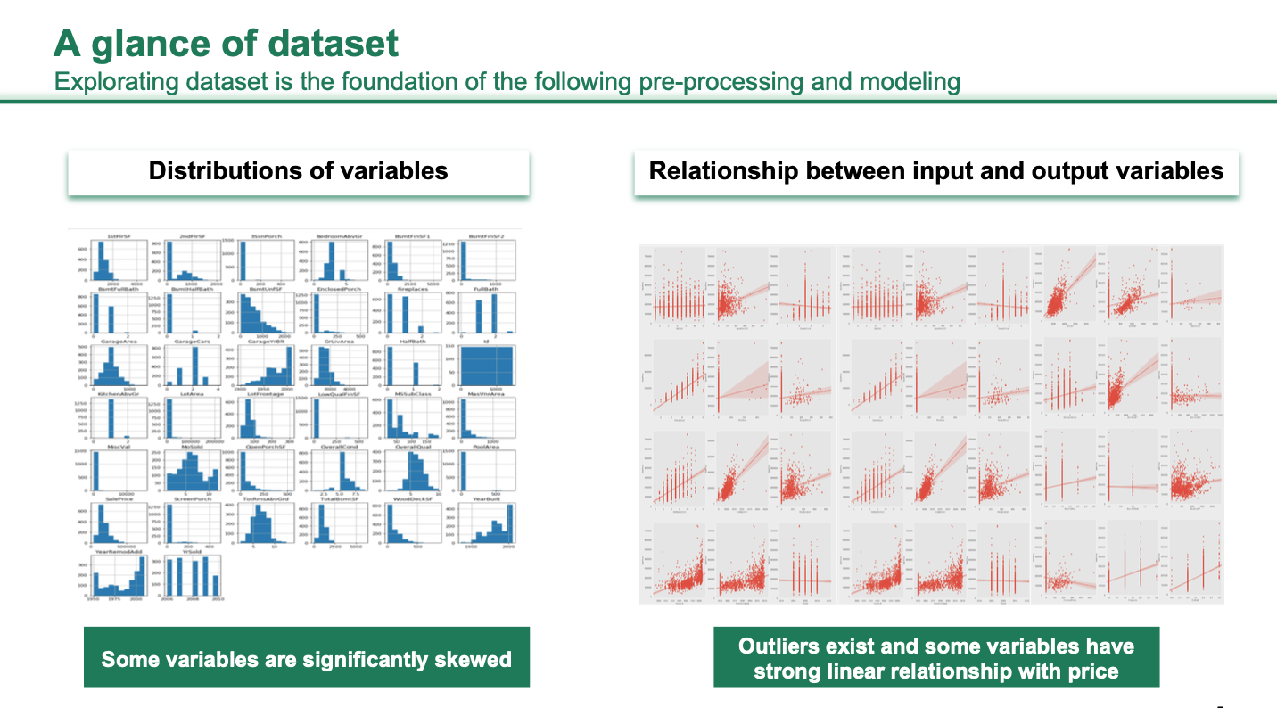
Understanding the dataset by visualizing the distribution of variables and their correlation with the target variable, we removed outliers and transformed the target variable. As can be seen in the plots below, outliers exist, and some variables have a strong linear relationship with the target variable.
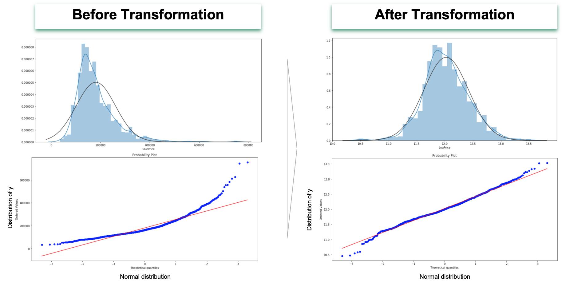
Log Transformation of Dependent Variable
A histogram and probability plot shows a left-skewed distribution curve of the dependent variable sale price with most of the houses being sold at the $100,000 to $200,000 range, as shown in the left plots below. The left skewness is caused by a small number of expensive houses and a concentration of cheap houses. To make this distribution more symmetrical, we took a log on the sale price, as demonstrated in the right plots. The rationale behind the log transformation on the target variable is as follows:
- It allows a non-linear and thus a quite general relationship between variables for having a multiplicative form.
- Sale price is always greater than or equal to 0, which makes it a limited dependent variable that needs particular techniques to address it. However, the log of it has a maximum value of positive infinity and a minimum value of negative infinity that averts the need for those techniques.
- It can reduce the effect of extreme outliers.
- If we have a model that has heteroscedasticity / non-constant variance, the log transformation will suppress the variation in the target variable and therefore reduce the heteroscedasticity.
- Similarly, it can also make the error's distribution more symmetric for the sake of normality assumption in linear regression.
Removing High Influential Points in Features that are Highly Correlated with the Target Variable
High influential points are the points that are both an outlier and having high leverage. An outlier is a data point whose response does not follow the general trend of the rest of the data. A data point has high leverage if it has "extreme" predictor values.
High influential points can't represent the general pattern of the data. They will pollute the linear regression model by 'dragging' the fitting hyperplane 'up' or 'down,' making the model either overestimate or underestimate the actual coefficients and intercept. This can particularly manifest in the predictor variables that are highly correlated with the response variable as they are more likely being influential to the prediction with higher coefficients.
Therefore, we filtered out the highly correlated predictor variables and identified and removed the influential points in these variables.
Imputation of Missing Values
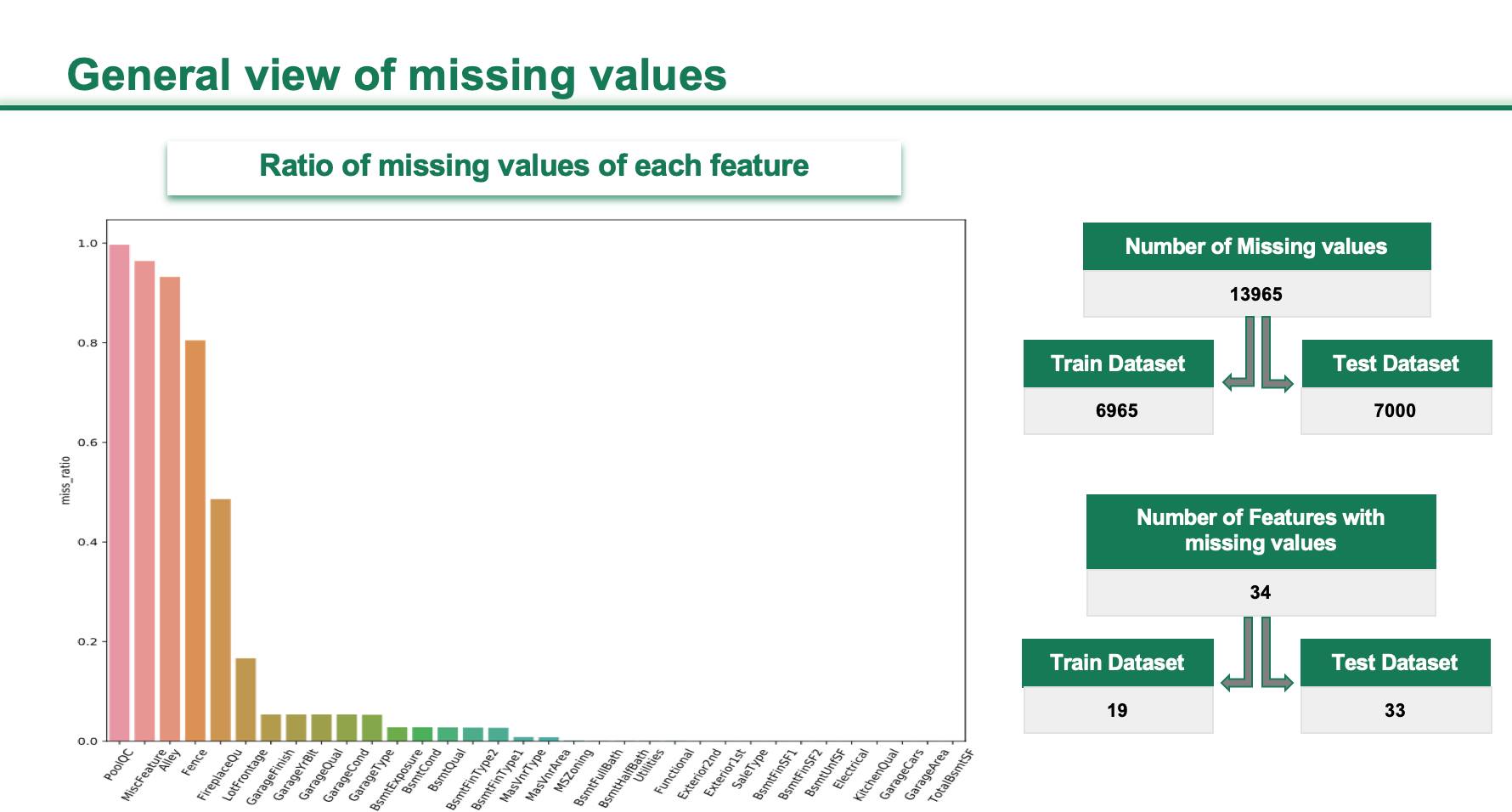
Overall, 6% of data was missing, and this occurred in 34 variables of the total 79 predictor variables. Four predictor variables have over 80% of missing value.
The number of variables with missing value in the test dataset is much greater than in the training dataset. The imputation has to be implemented in both the training and testing datasets. Let's take a look at our imputation strategy over the training dataset.
We identified missing values into 'pseudo' and 'real' missing values. The pseudo means the values are not actually missing. Instead, they are indicating a house without the corresponding attribute. For instance, the NaNs in variable PoolQC, which stands for swimming pool quality, represents houses without a swimming pool, which is common.
So we imputed these pseudo missing values with words/strings like 'No PoolQC.' For the real missing values, we imputed by grouping the values in the predictor variable by their labels in the related variable, taking the mean, median, or mode from the grouped values of the predictor variables, and using that to impute a missing value for predictor variable in each of the groups.
For example, we imputed 'LotFrontage,' which stands for the Linear feet of street-connected to the property by grouping the values in it by the labels of their corresponding Neighborhood, taking the median, and using it to impute. We also used some life experience and domain knowledge to impute. For example, we imputed the feature 'Electrical' by the industrial standard Electrical system ('Standard Circuit Breakers & Romex').
Similarly, we imputed the test dataset.
Feature Engineering
As our linear model is not robust enough to deal with different data types, we grouped the data into different categories: continuous, ordinal categorical, and nominal categorical, and transformed them respectively, as shown in the slide below.
When dummifying, every category will form its own column. However, many will not be numerous enough or different enough to form meaningful variables, like the 'Wall', 'OthW', and 'Floor' in the plot below.
So we grouped them as follows:
As the optimal situation to apply linear regression model on the data is that residuals/errors are normal, transforming both predictors and the target variable to more symmetric distribution can make our model more robust in the sense of statistical inference. Therefore, we applied a box-cox transformation to skew data that exceed a threshold of skewness.
In addition, we also created new variables based on our understanding of the data and domain knowledge. For instance, we add one feature, which represents the total square feet of the house:
attri['TotalSF'] = attri['TotalBsmtSF'] + attri['1stFlrSF'] + attri['2ndFlrSF']Model Fitting
We first trained a Lasso Regression Model and got a minimum test RMSE 0.1075 by selecting the optimal lambda. Then we performed feature selection using the optimal lambda to drop features that the corresponding coefficients are shrunk to 0. 119 features are dropped in total in both training and test datasets.
After that, we retune the lambda for the updated training dataset using Lasso and Ridge. After feature selection above and got a slightly better result (RMSE) in Lasso.
And a significant improvement in Ridge.
We also train Elastic Net Regression Models and found that Lasso returns us the best result among the three.
Lastly, we trained the other two models that are gradient boosting and extreme gradient boosting machine. And we stacked all the regressors by giving them different weights based on their least RMSE. Eventually, we got the best result: 0.1049 in RMSE.
This model achieved an average error of 4% within the most common price range from $50,000 to $20,0000.
Feature Importance
The top 10 predictor variables given by the feature importance score of gradient boosting machine are:
- TotalSF - Featured variable: Total Squared Feet of the house;
- OverallQual: Rates the overall material and finish of the house;
- GrLivArea: Above ground living area square feet;
- YearBuilt: Original construction date;
- KitchenQual: Kitchen quality;
- TotalBsmtSF: Total square feet of basement area;
- GarageArea: Size of garage in square feet;
- YearRemodAdd: Remodel date (same as construction date if no remodeling or additions);
- ExterQual: Evaluates the quality of the material on the exterior;
- 1srFlrSF: First Floor square feet;
Introduction to our Team
Author of this blog: Fred Lefan Cheng.


