Studying Data to Predict House Sales
The skills the author demoed here can be learned through taking Data Science with Machine Learning bootcamp with NYC Data Science Academy.
“Half the money I spend on advertising is wasted; the trouble is I don't know which half.”
– John Wanamaker
The sale of a house is a valuable event for many parties. Real estate brokers, mortgage originators, moving companies – these businesses and more would greatly benefit from being able to get out in front of their competitors in making contact with prospective home sellers. But who are these prospects? Data shows only one in 20 houses goes up for sale every year, so 95% of all households in a given year are not potential customers!
A company called SmartZip spent seven years building out analytics to predict who will soon put their house up for sale; my project was to accomplish a similar goal in three weeks using publicly available data.
Why Sell?
The first step was to identify what a homeowners may consider or be affected by when deciding to sell their house. The below diagram illustrates what I considered to be the key factors. Obviously, it is not possible to directly measure many of these dimensions, so I had to resort to using proxy values to approximate the true values. I also excluded some items from the study due to time constraints.
Data Procurement and Cleaning
Procuring all the data for this study was a bottleneck. Tidy data sets are readily available for academic use or sometimes available (for a fee) from data vendors. However, cobbling your own data set together across multiple data sources can be a bear of a task -- this project was no exception.
The below graph illustrates the data procurement process. All in all, I sourced five different data sets via a combination of two web scraping apps, one API, and a few flat files. Zillow proved to be the bottleneck because their API did not provide the historical data I needed and their site makes extensive use of AJAX calls, which means I had to use the comparatively slow Selenium instead of Scrapy.
All in all, I managed to get only 10% of the number of observations I had planned on working with. However, when considering the ratio of observations to features, the project was still viable. Below is a summary of the data set:
- 18,000 observations after cleaning
- 2,500 houses
- 10 years of observations
- 2 zip codes from different counties in North Carolina
- 61 variables => 24 features
- Unbalanced: 5% of houses sell in a given year
Data Missingness
Missingness was an important issue with this dataset. I ignored certain missing items, such as a house not being available on Zillow, under the assumption that they item got dropped for technical reasons in the web scraping process. But others I was less confident about. For example, I sourced addresses from a voter registration database. Therefore, households that do not contain at least one registered voter were implicitly excluded from the data set. If there are links between voter registration rates and other features in this data set – which isn’t hard to imagine – this form of missingness may bias the results.
| Missing Item | Type | Action |
| House profile not accessible on Zillow | MCAR? | Omitted |
| Square footage | MNAR/MCAR | Regression on number of bedrooms |
| Inadequate sale data | MNAR? | Omitted |
| Address not available in census | MNAR? | Omitted |
| Others | MCAR | Mean/median |
The general theme was that the quality of data decreases for older events. There was an especially insidious trend due to a combination of the increasing sparsity of historical transactions in Zillow and a particular type of filtering I had to perform regarding house values. The below boxplots reveal that in 2001 the data suggest all houses were being resold on a yearly basis – clearly not a possibility. To mitigate against this, I restricted the study to more recent years.
House Values
I wanted to account the fact that when deciding to sell, a person may consider the potential sale price of their house versus what they paid for it. Notions of sunk costs and inflation-adjusted dollars aside, psychological research has clearly illustrated that people anchor on numbers such as the purchase price of their house and often will resist selling until they can “get their money back”.
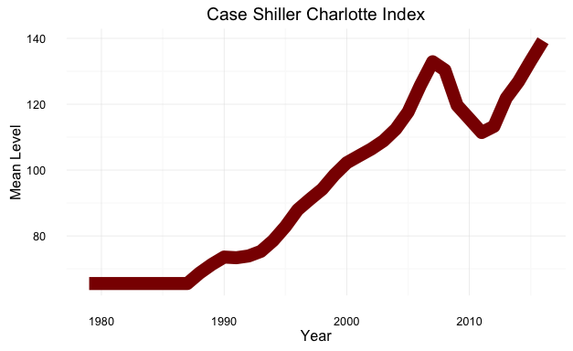
Unfortunately, housing is an illiquid market, and the tr ue value of a house is only revealed at the time of sale. To impute the value of a house for years in which it did not change hands, I applied the log returns of the Case Shiller Charlotte Home Price Index to the most recent sale price.
I also calculated an adjusted value based on how incorrect my Case Shiller index method was at estimating the values of houses that actually did sell in a given year. This served to periodically "re-center" an estimation based on related observations.
Data Analysis
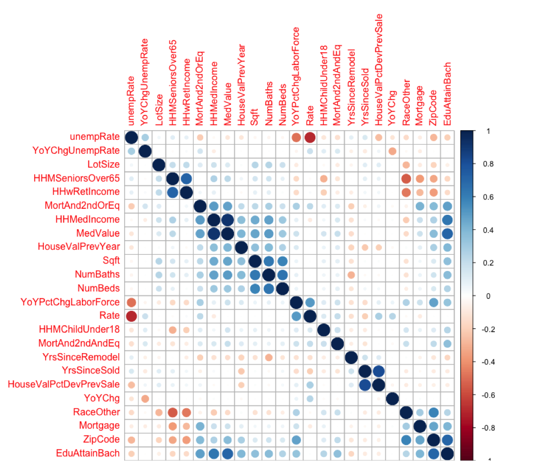
Compared to the preparation steps, the actual analysis of the cleaned data set was mercifully straightforward. The feature set looked fairly robust:
There is a cluster of moderate collinearity related to socioeconomic status, e.g., better educations with higher salaries in more expensive houses. And there are a few features that could potentially be dropped, such as unemployment rate versus mortgage rates. Otherwise, the features look OK.
Regression Results
Logistic regression showed many of the features’ coefficients where significant, but not all of them were behaving in an intuitive way:
From logistic regression I then proceeded to random forests. This model is useful because it is fast and easy to train. Moreover, it is robust to outliers and can capture non-linear relationships. Therefore, if random forests greatly outperformed logistic regression, I could prioritize feature engineering to help improve logistic regression’s predictiveness while still retaining its descriptiveness.
Unfortunately, this was not the case -- random forests did not have improved predictive ability. Additionally, the tree-based methods required oversampling to work at all with such an unbalanced data set. In the end, random forests, logistic regression, and XGBoost all had similarly poor predictive power, and feature subsetting or regularization did not make any material improvements.
Random Forest
The below ROC chart of each model’s performance shows that the AUC is not exceptionally large for any of them. The curve that slightly underperforms is of random forest's predicitions.
However, shooting for near-perfect accuracy isn’t really feasible when it comes to predicting houses going up for sale. The only infallible way to know if someone is going to sell is to knock on their door and ask them. But this is exactly the kind of unfocused allocation of resources this project is designed to prevent! Realistically, all we can hope for is to improve salespeople’s odds of spending time and money on actually prospects. To that end, the logistic regression’s results are, indeed, useful.
Distribution
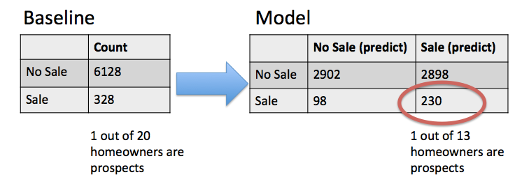
The above histogram illustrates the respective distributions of the houses put up for sale versus not against the probability of sale as per logistic regression. It’s clear that the distributions are not perfectly overlapping, as was evident in the ROC chart. By calibrating the cutoff on the logit function to yield a false positive rate of 0.5, we can greatly increase the true positive rate for a subset of households, as depicted in the below tables:
If a real estate broker were to use this model, they would be 60% more likely to distinguish prospects from non-prospects. All else being equal, that equates to 60% more revenue! Not a bad start for three weeks of work.
Going Forward
There are several enhancements I would like to make to this model in the future:
Broader rather than deeper
I used a large amount of historical data on a small number of houses because of the combination of time and technology constraints. It would be better to use a larger set of houses over a more recent time span. Historical patterns could instead be used to look for inflection points where next year’s sales may be less predictable based on this year’s data due to a potential change in macro factors.
Census block-level data
I also used census block group-level data rather than block-level due to time constraints. Block group-level is at a less granular level of aggregation than block-level data. Leveraging the block-level data may yield more accurate predictions.
Better estimates of housing prices
I would like to design a more precise house value estimator. Once I have a more dense population of houses, I will be able to regress house values on to contemporaneous sales of similar houses in the same area. This may make certain features more useful.
Mapping feature in Shiny
Once a good set of data is available, I would like to add a GUI that identifies high-probability addresses and integration with Zillow’s API.


