Using Data to Predict House Prices in Ames, Iowa
The skills the authors demonstrated here can be learned through taking Data Science with Machine Learning bootcamp with NYC Data Science Academy.
Data Science Introduction
Based on data over the past 50 years, a core pillar of achieving the “American Dream” is owning your own home. The importance of this life milestone is reflected by the sheer size of the real estate market:
- $35 trillion market at the time time of writing
- 25% of all households’ net worth is in the form of owner occupied real estate
- 15% of the American GDP is due to real estate-related spending
- 850,000 builders work in the residential construction industry
Buying a home is often the largest and most important purchase that most people will make during their lives. The process involves tradeoffs between what is desired, what is necessary, and what is affordable. Historically, determining the true value of a home has been something of a black box, as its market value is only revealed at the time of sale.
While real estate analysts have long used data to produce high-level, retroactive assessments about the housing market, the task of assigning values to individual homes before a sale has largely been left to appraisers, real estate agents, and sellers themselves. But times are changing. The confluence of big data and increased computing power are making the process of homebuying more transparent.
In this post, our goal as aspiring data scientists is to ease the stress of homebuyers making their purchases by shining through the cloud of price uncertainty with data science and machine learning techniques. We will provide a case study of how data science can add value to the home-buying process through highly practical and widely applicable machine learning models to accurately predict the sale price of homes in Ames, Iowa.
Data Overview
We used a data set made publicly available on Kaggle to build our prediction model. The dataset contains 1460 observations of homes sold in Ames, Iowa, between 2006-2010. For each home, there are 80 features, of which 33 are continuous, 14 are ordinal, and 33 are categorical.
Missingness
Around 6 percent of the data was missing, and of this missing data, most of it was ‘missing’ for a reason. Any variable related to a home’s basement or garage with a missing value meant that this home did not have a basement or a garage, so missing values for these features were imputed as 0. Other variables with missing values were imputed by finding the mode or mean value of the missing variable among other similar houses.
For example, 4 houses were missing values for zoning, so we imputed these values by finding the mode zoning value for other homes in the same neighborhood. Likewise, for the one home that did not have a value for the size of its masonry veneer, we found the mean veneer area of all homes that were built with the same veneer material.
Using Data to AnalyzeOutliers
Linear models are not robust to outliers, meaning one outlier could influence the true relationship between the house price and the predictor significantly. Therefore, we removed any observation that was 5 or more standard deviations away from the mean sales price relative to any particular variable. We created scatterplots to complement and confirm our decision to remove outliers from our model.
Feature Engineering
Using Data to Analyze Continuous Features:
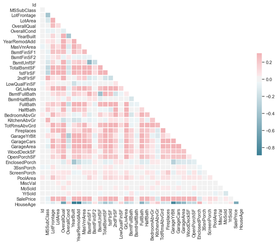
To begin, we looked at which continuous variables were the most correlated with our response (housing price) via a correlation heatmap:
We kept this in the back of our minds for the rest of the variable selection process, as a guide towards which variables might exhibit high multicollinearity and as a sanity check for which variables might be dropped by Lasso (more on this below).
We reduced the number of continuous variables to 19 by combining or features that expressed related or redundant information. For instance, there were 4 separate variables that reported the number of bathrooms in a home – full bath, half bath, basement full bath, and basement half bath.
We combined these 4 features into a single variable that expressed the total number of bathrooms. We followed a similar process to create custom variables for the total square footage of the basement and of the total outdoor living areas (porches). We also created a custom variable for the house’s ‘age’ that considers the year a house was built, remodeled, and sold
Lastly, in order to normalize our data, we took the log of each home’s sale price and used this variable in our machine learning models explained further down.
Using Data to Analyze Ordinal Features:
Of the 14 ordinal features’ scales, 4 were numeric, but 10 were represented by strings (e.g. excellent, good, average, fair, and poor). For each of these 10 features, we converted their strings to numeric values so that these features could be used in our linear regression model.
Using Data to Analyze Categorical Features:
The last group of variables that needed to be modified were the categorical features. After our initial exploratory data analysis, we dummified the most significant categorical values so that they, too, could be used in our model. Now that our data had been cleaned, we began building the model.
Using Data to Analyze Machine Learning Models
Our feature engineering resulted in a total of 99 variables to be used in our model. While we were intentional in selecting variables that both described distinct aspects of a house and appeared to have the most significant influence on a house’s price, we used two techniques – Variance Inflation Factor (VIF) and Lasso regression – to eliminate as much multicollinearity between features as possible. We want to do this because multicollinearity causes the estimates of our coefficients to become unstable and causes the model to generalize poorly on new, previously-unseen, data.
After computing our features’ VIF, we dropped two features that were highly correlated with other, more significant features, such as garage cars (highly correlated with garage area), and total number of rooms (highly correlated with size of living area).
Using Data to Analyze Lasso
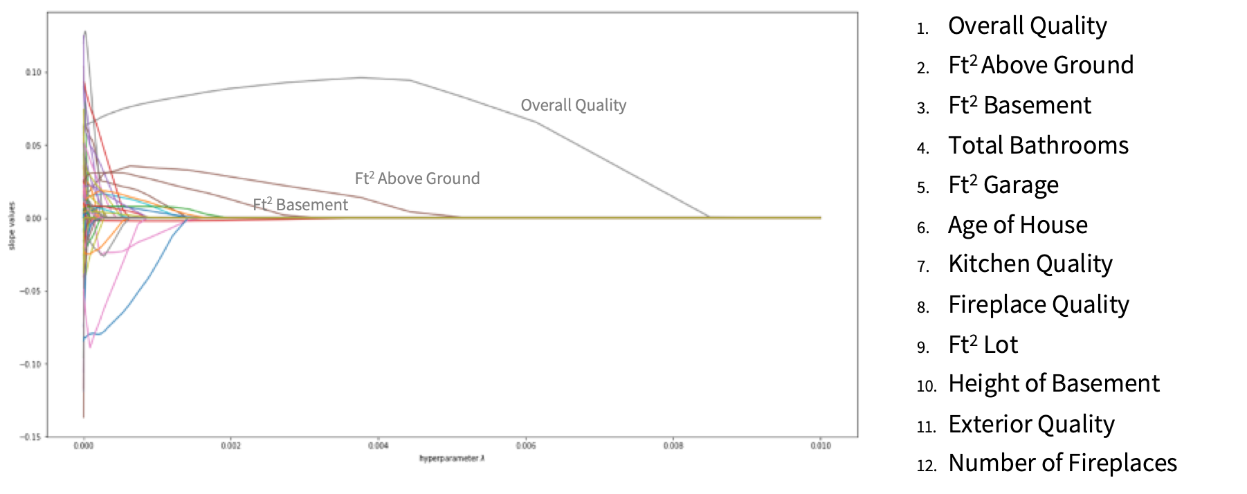
We used Lasso both to eliminate features with high multicollinearity and to create a predictive model. Lasso is a kind of regularized linear regression that captures the linear relationship between target variables and predictors. Compared with multiple linear regression, Lasso produces slightly biased linear models with much less model variance to achieve a higher predictive accuracy. The root cause of the high model variance is multicollinearity among features, which could result in over-estimated coefficients when applying multiple linear regression. Lasso fixes this problem by penalizing the model using a hyperparameter lambda.
Lambda controls the amount of penalization applied to the model. As lambda increases, it aggressively penalizes variables in the model, driving the coefficients for less important features to zero. However, we also want the model to contain as much information as possible and that is why we need to find the optimal lambda so that we can keep a balance in between.
The figure above shows our features’ behavior in the Lasso model. The lines to the chart’s far left that quickly drop to zero represent features that are less important to a home’s price, and the lines further to the right of the chart are more significant. The list to the right of the chart shows the top-12 features that most significantly influence a homes price. After passing our variables through a basic Lasso model, we eliminated over 30 more variables that were highly correlated and did not have a strong influence on a house’s overall price.
Using the top 60 features from the Lasso feature selection, we tuned lambda through 80/20 cross validation. The chart below shows the error values associated with different lambda values.
The goal of choosing the optimal lambda is to find the one that gives the lowest error on the test dataset. From the graph above, we chose 0.000056 as the optimal lambda which is the lowest point on the blue curve. By applying the optimal lambda to the lasso model, we obtained an RMSE score of 0.133 on Kaggle.
Using Data to analyze Gradient Boost Method
Gradient Boosting Method (GBM) is a tree based machine learning model that can capture nonlinear relationships between the target variable and predictors. It follows a sequential procedure such that each tree uses information from previously grown trees, and the addition of each new tree improves upon the performance of the previous trees. In doing so, GBM converts many weak learners into strong learners and increases its predictive accuracy.
Compared to a linear model, a tree-based model requires much less data preprocessing. For example, GBM allows the transformation of categorical strings into numeric values through the process of label encoding, as opposed to a Lasso model which requires dummification and results in extra columns with sparse information. Additionally, tree-based models are not sensitive to the scaling of input features, so log transformations or normalization are not required for tree-based models.
After data preprocessing, the data we fed to the GBM model contained 82 columns including both continuous and ordinal features.
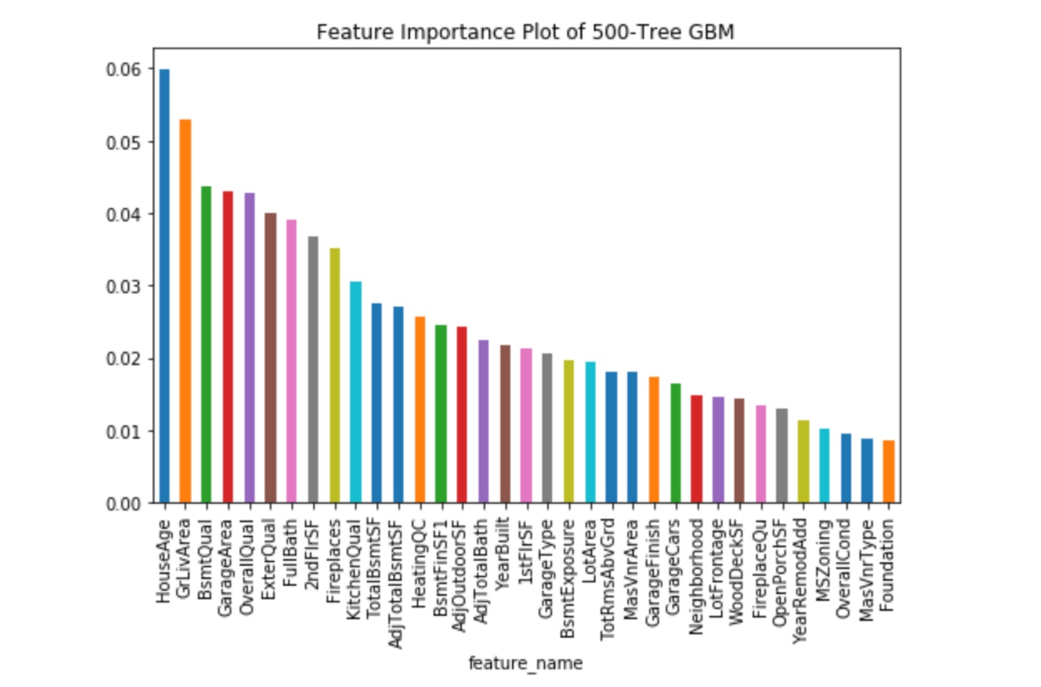
The figure above shows the top 35 features in the order of feature importance ranked by the GBM model. It suggests that the age of the house, sizes of the living area, basement and garage, as well as the overall quality of the house have the strongest impact on a house price. Some other features such as number of bathrooms, kitchen quality and neighborhood also influence a house value.
Among the features over which homeowners have partial or total control over, the ones ranked at the top are: age of the house, basement quality, and kitchen quality. This implies that home renovations such as finishing the basement or installing granite countertops in the kitchen, may produce the highest return on investment, when the homeowner is ready to sell the house.
With these 35 features, we tuned the hyperparameters and obtained an error score of 0.135 on Kaggle.
Using Data to analyze Bayesian Ridge
Bayesian Ridge is a machine learning model that doesn’t try to find the “best” value of model parameters, but rather, it tries to determine the posterior distribution of the model parameters, which is conditional on the training inputs and outputs. It is similar to Lasso regularization, in the sense that it also balances between removing redundant features vs keeping enough features to accurately predict housing prices. However, it has many more hyperparameters to tune. The implementation in Python has four hyperparameters to tune, which takes a longer time to train through cross validation.
The inputted data that we used contained 99 columns in total, which includes continuous, dummified, and ordinal features. After tuning our Bayesian Ridge model, we obtained a 0.1324 error score on Kaggle.
Using Data to Analyze Ensembled Model
In the 2004 book The Wisdom of Crowds, author James Surowiecki presents cases in economics and psychology where the collective estimates generated by crowds outperform those of any single individual. In this book, the opening example was: the crowd at a county fair accurately guessed the weight of an ox when their individual guesses were averaged (the average was closer to the ox's true butchered weight than the estimates of most crowd members).
Data science often applies a similar concept – combining many weaker learners generates a strong learner. We created an ensemble of three models. By using a weighting of 25% Lasso, 40% GBM, 35% Bayesian Ridge, we obtained a Kaggle score of 0.1241, which is superior to any of the individual performances of the models, and this RMSE ranks in the top 20% of Kaggle scores.
While an ensemble model trades increased accuracy for decreased interpretability, if the goal of the client is to simply obtain the most accurate price prediction for a house, an ensemble model is the best model to use.
Conclusion
Using a data science pipeline consisting of EDA, imputing missing values, removing outliers, feature engineering, transforming predictors, and ensembling linear and nonlinear machine learning algorithms, we managed to:
- Score in the top 20% ranking of Kaggle competitors for this dataset, which delivers accurate price predictions to help homebuyers gauge how high they should bid
- Understand which features are the most significant in determining the value of a home, which is useful for homeowners seeking to increase their home’s resale value through renovations
Given the amount of data available, the possibilities for our next project in applying data science to the real estate market are virtually endless. In future work, we could expand upon our existing foundation by:
- Including data on non-traditional factors such as the number of cafes within a defined radius to augment models and make more accurate housing price predictions
- Building recommender systems to suggest properties that match homebuyers’ purchasing needs and financial goals
- Making forecasts that develop and refine indices to accurately predict property prices many years in the future
We are excited to work together with you on further data science projects, within the real estate domain, or to other areas of business, given that the techniques that we used here are universally applicable and mostly domain-agnostic. Our contact information is listed below – do feel free to get in touch.
Joe Lu - Linkedin / Github / Email
Jordan Runge - Linkedin / Github / Email
Yunmei (May) Zhang - Linkedin / Github / Email
Xuyuan (Alice) Zhang - Linkedin / Github / Email


