Walmart Kaggle: Trip Type Classification
Contributed by Joe Eckert, Brandon Schlenker, William Aiken and Daniel Donohue. They took the NYC Data Science Academy 12-week full-time data science bootcamp program from Sep. 23 to Dec. 18, 2015. The post was based on their fourth in-class project (due after the 8th week of the program).
Introduction
Walmart uses trip type classification to segment its shoppers and their store visits to better improve the shopping experience. Walmart's trip types are created from a combination of existing customer insights and purchase history data. The purpose of the Kaggle competition is to use only the purchase data provided to derive Walmart's classification labels. The goal for Walmart is to refine their trip type classification process.
About the Data
- ~ 96k store visits, segmented into 38 trip types
- Training and testing data included >1.2 million observations with 6 features:
- Visit Number, Weekday, UPC, Scan Count, Department Description, Fineline Number
- Using the 6 provided features the team was tasked with creating the best model to accurately classify the trips into their proper trip type category
- Challenges with the data
- Each observation represented an item rather than a visit
- Needed to group observations by visit to classify the trip
- Number of unique UPCs and Fineline Numbers prevented the creation of dummy variables - resulting data set was too large to process
- Instead, used the Department Description to create dummy variables
Model 1: Logistic Regression
Implemented multinomial logistic regression to determine trip type. Normal logistic regression is used for two class predictions. Multinomial logistic regression performs logistic regression on each class against all others. The process is repeated until all classes are regressed one vs all.
- Log loss score: 4.22834
import pandas as pd
import numpy as np
import scipy as sp
from sklearn.linear_model import LogisticRegression
import time
start_time = time.time()
waltrain = pd.read_csv('train.csv')
waltest = pd.read_csv('test.csv')
waltrain = waltrain[waltrain.FinelineNumber.notnull()]
waltrain_part = waltrain[:]
waltest_part = waltest[:]
model = LogisticRegression()
x = waltrain_part[['Weekday', 'DepartmentDescription']]
y = waltrain_part[['TripType']]
x = pd.get_dummies(x)
z = waltest_part[['Weekday', 'DepartmentDescription']]
zend = pd.DataFrame({'Weekday': ['Sunday'],
'DepartmentDescription': ['HEALTH AND BEAUTY AIDS']},
index = [len(z)])
z = z.append(zend)
z = pd.get_dummies(z)
model.fit(x, y)
print "The model coefficients are:"
print model.coef_
print "The intercepts are:"
print model.intercept_
print "model created after %f seconds" % (time.time() - start_time)
submission = model.predict_proba(z)
submissiondf = pd.DataFrame(submission)
submissiondf.drop(len(submissiondf)-1)
dex = waltest.iloc[:,0]
submurge = pd.concat([dex,submissiondf], axis = 1)
avgmurg = submurge.groupby(submurge.VisitNumber).mean()
avgmurg.reset_index(drop = True, inplace = True)
avgmurg.columns = ['VisitNumber', 'TripType_3','TripType_4','TripType_5','TripType_6','TripType_7',\
'TripType_8','TripType_9','TripType_12','TripType_14','TripType_15','TripType_18',\
'TripType_19','TripType_20','TripType_21','TripType_22','TripType_23','TripType_24',\
'TripType_25','TripType_26','TripType_27','TripType_28','TripType_29','TripType_30',\
'TripType_31','TripType_32','TripType_33','TripType_34','TripType_35','TripType_36',\
'TripType_37','TripType_38','TripType_39','TripType_40','TripType_41','TripType_42',\
'TripType_43','TripType_44','TripType_999']
avgmurg[['VisitNumber']] = avgmurg[['VisitNumber']].astype(int)
avgmurg.to_csv('KaggleSub_04.csv', index = False)
print "finished after %f seconds" % (time.time() - start_time)
Model 2: Random Forest
For the second model the team implemented a random forest. Random forests are a collection of decision trees. Classification is done by a 'majority vote' of the decision trees within the random forest. That is, for a given observation the class that is most frequently predicted within the random forest will be the class label for that observation.
Engineered Features:
- Total number of items per visit
- Percentage of items purchased based on Department
- Percentage of items purchased based on Fineline Number
- Percentage of items purchased by UPC
- Count of different items purchased (based on UPC)
- Count of returned items
- Boolean for presence of returned item
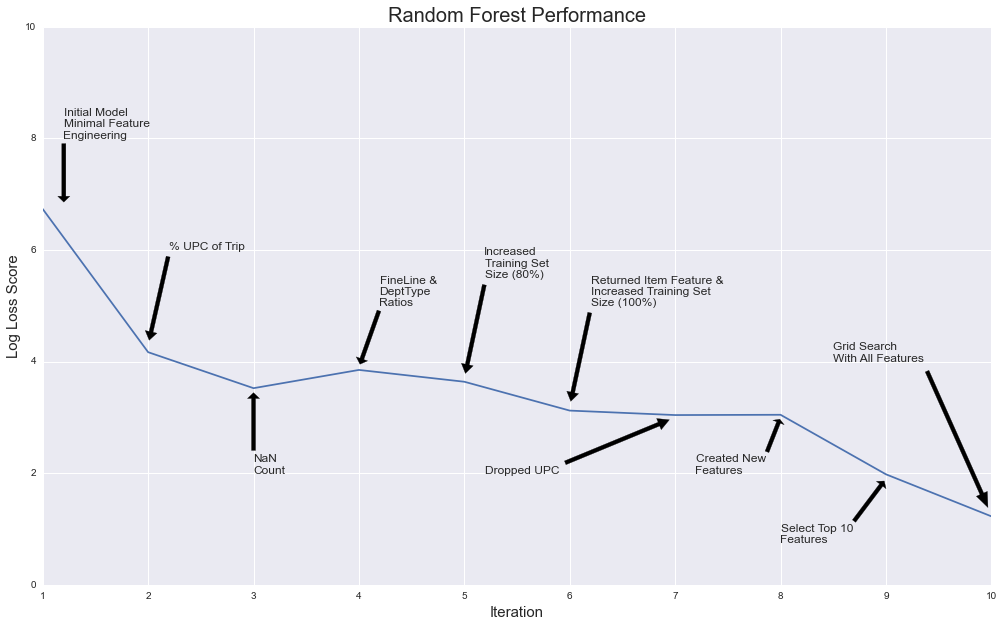
Below you can see the progression of the performance of the random forest as adjustments were made:
- Best log loss score: 1.22730
Model 3: Gradient Boosted Decision Trees
Gradient boosted trees are a supervised learning method where a strong learner is built from a collection of decision trees in a stagewise fashion, where subsequent trees focus more on observations that were misclassified by earlier trees.
Engineered Features:
- Day of the week (expressed as an integer)
- Number of purchases per visit
- Number of returns per visit
- Number of times each department was represented in the visit
- Number of times each fineline number was represented in the visit
For this model the team used the XGBoost and Hyperopt Python packages. XGBoost is a package for gradient boosted machines, which is popular in Kaggle competitions for its memory efficiency and parallelizability. Hyperopt is a package for hyperparameter optimization that takes an objective function and minimizes it over some hyperparameter space. Unfortunately, we needed to split the training set into two halves (the prepared dataset was too large to keep in memory), train two XGBoost models, and then average their results. Not training on the whole dataset is probably what resulted in the larger log loss score.
- Best log loss score: 1.48
The code for this approach to the problem can be found here.
Conclusion
Given the size of the data set the accuracy achieved was limited due to memory constraints. The best performance was achieved using random forest after implementing grid search for feature selection and parameterization. Feature engineering was extremely important in this competition given that the rules restricted the use of external data.


