Data Analysis Ames Higher: House Price Prediction
The skills I demoed here can be learned through taking Data Science with Machine Learning bootcamp with NYC Data Science Academy.
Our project aims to investigate a dataset of house sales in Ames, Iowa, and use it as a basis to generate an interpretable and accurate machine learning model to predict house prices. The dataset for this analysis comes from the Ames Assessor’s office, taken from Kaggle, and includes information on 1,460 house sales from 2006 to 2010 including 79 descriptors of the house, the property, and the surrounding area.
What defines the price of a house?
We considered the question of defining the price of a house from two angles: our own opinions as potential buyers and aspects possibly important for a real estate agent.
Buyer
- Living Space (size)*
- Property (size)*
- Quality
- Neighborhood
- Curb Appeal*
- Good schools, safety
- Future resale potential
- Required Maintenance
- Close landmarks/parks/amenities
- Full-size Halloween candy
Real Estate Agents
- Price of comparable houses sold*
- Supply and demand*
- Interest rates
- Macroeconomic factors:
- Consumer Confidence
- Economic growth
- Demographics
- School system
- Property taxes
With these concepts in mind, we had a careful look at the data to determine which of these putative predictors were provided in the dataset and which ones we could design based on the details provided in the dataset. While features such as house quality, neighborhood, age and proximity to certain amenities were readily available in the dataset, we were also able to design additional possible house price predictors (indicated above with an asterisk).
Understanding the data
However, before applying mathematical models for house price predictions, we first needed to carefully analyse the dataset starting with missing information. 19 of 79 columns containing different property information contained some level of missing information. Some of these were highly correlated with other information provided. For example columns with detailed information on basement features contained no values for properties without a basement.
Similarly, specific garage features only included information for properties that had a garage. However, one important feature with a large proportion of missing information (17.8%) was lot frontage (street length in feet connected to property). We realized that different neighborhoods differed significantly in their property sizes and lot types (indicated by lot configuration).
We, therefore, imputed the missing values for lot frontage with the mean lot frontage of houses in the same neighborhood and with the same lot configuration. Where information about lot configuration was unavailable the mean lot frontage of the respective neighborhood was used.

We then investigated the dataset in more detail, in order to identify columns that contained overlapping information and those that would provide information for possible predictors as defined above (feature reduction and feature engineering). One example of feature reduction is porch size. The dataset contains information on the length of porches categorised into 5 different porch types.
Porch Types
Interestingly, a significant number of houses had several porch types listed. We decided to combine these into a single column of porch size and drop the individual porch type columns. Similarly, we decided to combine the basement and above ground bathrooms into a total number of bathrooms. An example of a new possible predictor we generated was “Neighborhood Building Type”.
New Column
This newly created column was calculated using an average price per sqft of similar houses in the neighborhood using KNN. For more details on our feature reduction and engineering, please have a look at our github repository.
With this data analysis in place, we decided to see how well ten intuitively chosen features would be able to predict house prices in a multiple linear regression model. The ten predictors we chose were: living area, building type, house style, overall quality, overall condition, condition 1 (proximity to main roads, railway, park,..), condition 2, lot area, year remodelled, and neighborhood.
Interestingly, this intuitive model explains 89% of the variance in sale prices, with increases in the overall condition by one category leads to a 3.7% increase in house price and proximity to railroads reducing the price by 9 - 23%, all else being equal.
Modelling
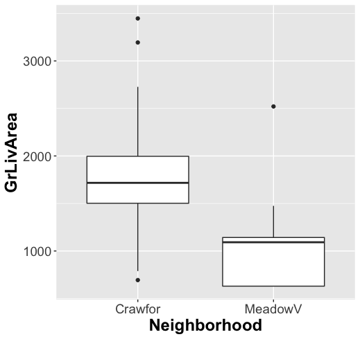
To help us gain a better understanding of our features we fitted a lasso regression model, which explained 94% of the variance using 52 features. Among those features were neighborhood, with Meadow Village and Crawford being two of the strongest predictors of the sale price. This makes intuitive sense but we ultimately decided to exclude neighborhoods from our practical regression model we found the neighborhood feature to be highly correlated with living area in our dataset.
We were able to reduce the number of variables without affecting the precision of the model significantly. Some of the variables we decided not to include were the lot area, the year of construction and house style, among others.
Some of the features that were included were:
- comparable price: where we used KNN to find the prices of similarly sized houses
- curb appeal: the product of masonry veneer area and lot frontage
- basement “niceness”: includes the basement square footage, quality and exposure,
- proportion of lot used
- sale condition
- roof material
Other models
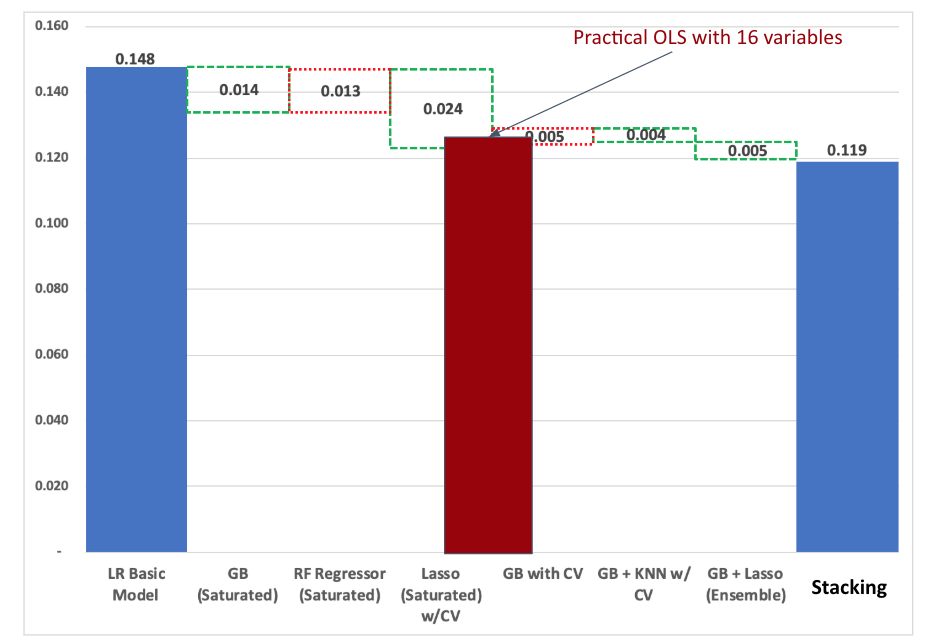
We also tried all linear models (simple regression, ridge, elasticnet), random forest, regression trees (CART), gradient boosting, XGBoost, KNN regressor and different versions of horizontal and vertical stacking. In addition, we applied different regression models for different house sizes which produced improved results.
Our best model in terms of RMSLE on the test set was an ensemble of 50% lasso and 50% gradient boost, putting our team in the top 15% on the Kaggle leaderboard. Overall, however, we found that the improvement in score over our practical model was trivial compared to the loss of explainability.
Interesting Observations
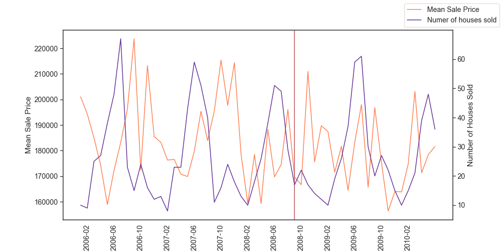
When we first started the project we had initial hypotheses about certain features in the data that we thought would be highly significant in our models. Since the dataset spans 2006 to 2010, we expected that the year a house was sold - whether it was pre or post the housing bubble - would have a considerable impact on the price.
Although the data shows a dip in the number of new houses sold and an increase in foreclosures, the overall impact on prices is trivial as shown in the figure below. This is also supported by the absence of the year sold feature from our lasso and ridge models.
The high variance of Sale Price for different Sale Conditions was another unexpected characteristic of the data. The difference in price between abnormal (mostly foreclosure) sales and normal sales is much smaller than the difference between normal sales and partial (mostly new) sales. Using different regression models for different sale conditions was initially considered, but due to the small proportion of non-normal sales in this data set we decided to leave it for further investigation.
Further Work
While our top-performing model was an ensemble of gradient boosting, elastic net, ridge and lasso, we ultimately decided to sacrifice the minute improvement in RMSLE for an interpretable linear regression model based on our research, intuition and feature importance outputs from other models.

We found that our linear models tend to overestimate cheaper houses, as illustrated by the residual plots below. In the future, we would like to explore using LOESS and/or spline regressions to dampen this effect.
Reevaluating outliers using techniques such as Hubert Regression and Z-Scores is another topic for further work as we relied on a Cook’s distance of 0.3 to filter out outliers.
Finally, for future projects, we think it would be more efficient to define tasks in terms of functions with clear inputs and outputs that team members can work on individually and that can be seamlessly integrated into a master script to avoid redundant and incompatible code.