Ames, IA Housing Price Predictions Using Data Pre-Processing and Machine Learning
The skills the author demonstrated here can be learned through taking Data Science with Machine Learning bootcamp with NYC Data Science Academy.
Introduction
The Ames Iowa Housing Project is a famous Kaggle competition that allows Machine Learning enthusiasts to truly flex their creative muscles. In this project, we’re given a dataset of 1,460 houses that were sold between 2006 and 2010. Also, this dataset contains an extremely rich amount of data on the makeup of each house — from the total square footage to the style of the roof.
Overview
In total, this dataset contains 81 variables about each individual house. The focus of this project is to train a machine learning model using the training data and predict what the final sale price of each house was in a separate test set, using all the factors at our disposal.
Someone new to Machine Learning may be tempted to ask, “Why don’t we just throw every variable into a multiple linear regression model and see what it outputs?”. The beauty of this dataset is that there is so much value and accuracy to be extracted from the data if you are willing to truly explore and manipulate it from the ground up.
Additionally, there are a variety of categorical variables that won’t be suitable for a multiple linear regression model, given that it only takes numerical values. Because of this, we’re forced to dummify, label encode, drop, combine, or do something else with all of our categorical variables.
Additionally, throwing all the variables into a model would not work, because this dataset is loaded with multicollinearity — or a tendency for multiple of our house features to be heavily correlated with each other. Multicollinearity is a big source of error within machine learning models, and justifiably so! If a large garage causes an increase in home value, but a large garage also tends to go hand in hand with a larger basement, then can we truly deduce that it’s the garage that is causing the increasing value, or is it the basement masked as the garage?
These types of problems are baked into the regression algorithms, and they can cause massive inflation of the standard error, and potentially lead to wildly inaccurate predictions. This is important to keep in mind as we explore our dataset.
Process - Pt. 1
To begin, I opted to drop all variables that contained over 85% of their points concentrated into a specific value. For example, the 3 Season Porch variable represents the area, in square feet, of each house’s 3 season porch. While a 3-season porch likely drives some value into a home’s overall price, 98.4% of our datapoints had a 3-season porch size of 0, signifying that they didn’t have such a porch.
With almost no variation in the values that our model can train from, I infer that there is more cost in including this variable than there is benefit. These costs include multicollinearity, as covered above, but also the curse of dimensionality, which causes models to categorize datapoints exponentially less effectively as the number of dimensions increase. In total, applying this 85% rule across all the features successfully eliminated 27 variables.
Next, I opted to remove columns with too much missing data. While there is value in imputing some missing data, trying to estimate too many datapoints can lead to a feature that is unreliable. This led to the removal of columns such as Alley access (93.8% missing data) and Pool Quality (99.5% missing data).
Process - Pt. 2
For the remaining columns that contained missing data, our approach largely featured utilization of KNN, or K-Nearest Neighbors. And, for any categorical variable that uses KNN to impute, the approach is simply to take each datapoint that is missing a value and see what characteristics a house of similar sale price has.
For example, the houses with a missing masonry veneer type were able to reference the houses that were sold for a similar price (the nearest 38 houses, to be exact, as we typically utilize the square root of our sample size to define K, and the square root of 1460 is about 38). Looking at the masonry veneer type of the “nearest” houses in terms of sale price, I was able to make a best estimate as to what the veneer type is. Even if I impute incorrectly, I can deem this generally more valuable for our model than removing either the house or the variable altogether.
An alternative to KNN for missing values is to encode missingness as a value to see if there is a trend in what kind of houses are missing a specific variable.
Process - Pt. 3
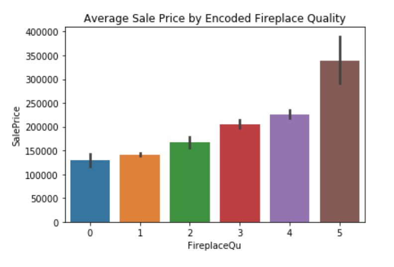
For the fireplace quality variable, I encoded houses with a missing quality as their own group and observed the average sale price of that group against all the other groups (poor, fair, average, etc).
By identifying a clearly positive and general trend among the quality categories, I opted to label encode these values numerically (poor maps to 0, fair maps to 1, average maps to 2, etc). What’s more, is that I was able to see that houses with a missing fireplace fall squarely within the linear sale price trend between houses of poor and fair fireplace quality. Thus, I re-encoded the variable so that 0 denoted a poor fireplace, 1 meant the fireplace was missing, 2 equated to fair, 3 meant averages, 4 meant good, and 5 meant excellent.
This approach of both encoding missingness and label encoding an entire variable is an efficient way to eliminate missing values from a dataset, as well as making categorical variables workable with regression. Of course, this particular feature of fireplace quality worked on an ordinal scale, in which there was an inherent order to the values. It gets trickier with nominal, less ordered features, but I can use similar methodology around encoding missing data when considering if I want to dummify other variables.
Process - Pt. 4
The bulk of the remaining preprocessing work came in the form of dealing with my categorical variables. As mentioned before, all values must be in a numerical form before regression modeling, which yields a multitude of routes I could go. For some variables, like the 2nd exterior material covering the house, I simply dropped the variable, due to having highly dispersed values, each of which would have to be label encoded into a number or into a separately dummified variable for me to use it. For other variables, like RoofStyle, I did go ahead with dummification, but with a more manually controlled approach.
In this instance, most of the values were concentrated into “Gable” and “Hip” style roofs, with 4 other roof styles dispersed among 33 other houses. After investigating each roof’s average SalePrice, I opted to dummify Gable roofs, Hip roofs, and “other” style roofs. Dummification, for reference, is the process of creating a brand-new variable, that simply points to the existence of a categorical variable for a given house.
Process - Pt. 5
If a house has a Gable roof, the dummified Gable column will have a value of 1, while all other dummified columns that refer to roof style will have a value of 0. I took a similar approach with the Masonry Veneer type variable, creating dummy variables of BrickFace Veneer, Stone Veneer, and other. Dummifying is extremely useful and powerful, but also requires extreme caution and moderation, so that the model doesn’t end up with excessive amounts of variables that could contribute to inaccuracy.
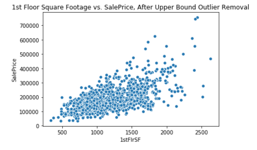
A model’s accuracy can also be heavily compromised by outliers, which tell a story in and of themselves. For example, our data shows a clear positive correlation between the 1st floor square footage of a home and its sale price, as one would expect. Why then, does the home with by far the largest 1st floor (4,692 square feet, with the next largest being 3,228) have a sale price of only $160,000, which is well below average?
We can’t know for sure, but I can infer that there is likely something wrong or incomplete with the condition of the house. These outlierish datapoints come up all throughout the dataset, and while it can be detrimental to remove houses from our dataset, it has more longstanding benefit to the accuracy of our model to drop the data altogether. For 1st floor square footage, for example, I dropped 4 such datapoints. Ultimately, after exploring our numerical variables, I found 28 outlierish datapoints that appeared to be worth dropping, leaving us with a training set of 1,432 points.
Process - Pt. 6
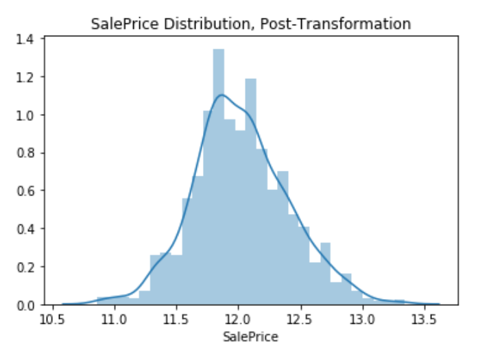
One of the last ways in which I manipulated the training data is by transforming our output variable, sale price. Regression functions at its best when data is not skewed, particularly with the variable in which we are trying to predict. By taking our sale prices and extracting the natural log of them, I reshaped the distribution of sale price to take on a much more Gaussian shape. To untransform this, all I’ll have to do is take each predicted sale price, and raise the mathematical constant e by that power, and I’ll have the final sale price prediction.
Before I could build models, I had to make the equivalent manipulations to our test set, so that the feature space matched the training set. Additionally, this test set came with some missing values, however it was very few; there were 6 missing values spread across 4 variables. Because these variables were all numerical, and the missingness was so light, I decided to simply impute these values with the mean value of those columns within the test set.
Process - Pt. 7
To actually build the models, I chose to move forward with a multiple-linear regression, a lasso regression, and a ridge regression. For the multiple-linear regression, I chose to first try building a model with a train-test-split, so that I could check for overfitting. Since that model yielded a minimal difference in accuracy between the training and test set, I decided to train an additional model on the entire dataset, so that the algorithm had the benefit of utilizing the full sample of training points. Since overfitting wasn’t a huge problem, I could have stopped with this model, but I decided to try regularized regression as well.
For both Lasso and Ridge, I utilized grid search to find the ideal hyperparameters that would introduce a little bias to the training set such that it was more generally applicable to the test data, and random noise within the training data had less of an influence. Ultimately, both of those models ended up being less accurate than the multiple-linear regression model, which is most likely a result of the focused feature generation, feature manipulation, and outlier removal that took place in preprocessing.
Conclusion
All in all, this project serves as a great way to not only gain a grasp of the fundamentals involved with cleaning a dataset for machine learning, but it allows you to find your own style and unique approach to data preprocessing and model building. From dummification, to label encoding, to KNN imputation, to encoding missing values, as well as a multitude of other approaches and combinations of the above, machine learning accuracy truly has the ability to shine when the model creator puts thought, time, and creativity into the data cleaning.
Innovative approaches can often go sideways and have a very counterintuitive effect on model accuracy but given that we have very strong computational power which supports a process of trial and error, I would encourage anyone to try their own unique approach when using machine learning to predict housing prices and beyond!
Sammy Dolgin is a graduate of the NYC Data Science Academy and Loyola University Chicago's Quinlan School of Business. He can be contacted at sammydolgin@gmail.com. All code used within this project can be found here.


