Airbnb Data Analysis and Modeling of New York City
The skills I demoed here can be learned through taking Data Science with Machine Learning bootcamp with NYC Data Science Academy.
I. Introduction
Airbnb is an online-based marketing company that connects people looking for accommodation (Airbnb guests) to people looking to rent their properties (Airbnb hosts) on a short-term or long-term basis. The rentals properties includes apartments (dominant), homes, boats, and whole lot more.
Since its inception in 2008, Airbnb has steadily risen in terms of revenue growth and its range of service provisions. As of 2019, there 150 million users of Airbnb services in 191 countries, making it a major disruptor of the traditional hospitality industry (this is akin to how Uber and other emerging transportation services have disrupted the traditional intra-city transportation services).
Airbnb generates revenue by charging its guests and hosts fees for arranging stays: hosts are charged 3% of the value of the booking, while guests are charged 6%-12% per the nature of the booking. As a rental ecosystem, Airbnb generates tons of data including but not limited to: density of rentals across regions (cities and neighborhoods), price variations across rentals, host-guest interactions in the form of reviews, and so forth.
NYC Airbnb Market
New York city (NYC) has an extremely active Airbnb market with more than 48,000 listings as of August in the 2019 calendar year (this corresponds to a rental density of 48000 rentals per 468 square miles, which equates to 102 rentals per square mile). This project focuses on the gleaning patterns and other relevant information about Airbnb listings in NYC. To be more specifically, the goals of this projects are to answer questions such as: (i) how are rental properties distributed across the neighborhoods of NYC (there are 221 neighborhoods);
(ii) how do prices vary with respect neighborhoods, rental property types and rental amenities; (iii) more importantly, how well can machine learning models be trained to predict Airbnb rental prices using features such as rental property type, the number of people a rental can accommodate, the number of available beds, and so forth.
II. Data Set
The data was downloaded from Inside Airbnb: http://insideairbnb.com/get-the-data.html The data set that was employed was named listings.csv; it is a detailed data set with 106 attributes, a few of the attributes being: price per day (which will hereafter be simply referred to as price), number of beds, property type, neighborhood, cleaning fee, security deposit, host's ratings score, etc.
The data contains a total of 48,864 listings which spans a period of more than 90 months from August 2019. We discarded listings older than 12 months; we kept only listings posted within 12 months of August 2019. The reason for doing so is that that those prices are more recent and thus more realistic. This reduced the number of listings to 37,359.
III. Exploratory Data Analysis
We initially explored the data to gain some initial insights into the distribution of the various features. We will present a few here visual representations here.
Figure 1 depicts the frequency of each rental property. Clearly apartments, which comprise about 78% of the rentals, are dominant, with houses accounting for 10%.
Figure 2 depicts the average price per rental property in NYC. Water-related rentals (boats, lighthouses, resorts) are the most expensive. Apartments and houses, which comprise the most dominant listings, are reasonably priced on the average (approximately $180).
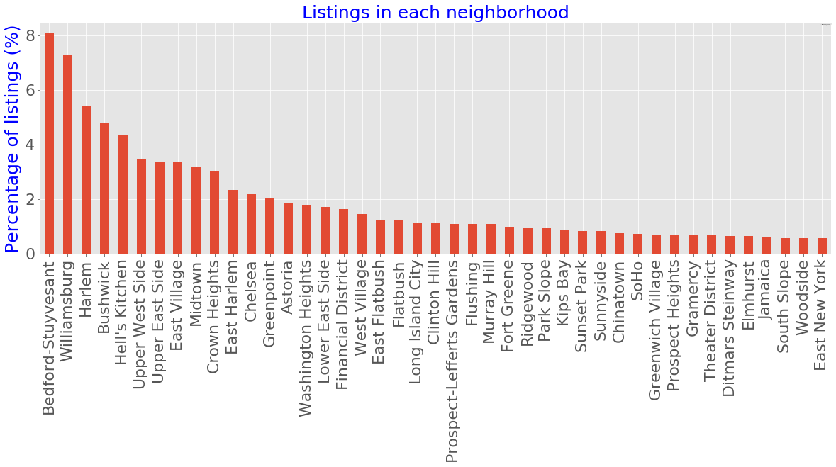
Shown in Figure 3 is the number of listings in each neighborhood within the past 12 months; Bedford-Stuyvesant is the neighborhood with the most listings (8.1%) followed by Williamsburg (7.3%). The figure shows neighborhoods with at least 200 listings; this corresponds to 43 out of the 221 neighborhoods. Collectively the 43 neighborhoods in figure 3 comprise 82% of the total listing.
Average price
The average price of rental properties in each neighborhood is shown in figure 4; only the top 40 average prices are shown in the plot. Comparing figure 4 to figure 3, it can be observed that there an inverse relationship between the average prices of properties and the number of listings in the neighborhood. For example: none of the three neighborhoods with the most listings in figure 3, namely Bedford-Stuyvesant, Williamsburg and Harlem, show up in the average price plot in figure 4.
Figure 5 depicts the distribution of prices with respect to room type. Majority of the private/single rooms are reasonably priced in the $50-$100 range, whereas majority of entire home/apartments lie in $100-$250 price range.
IV. Machine Learning Modeling
A. Feature Selection
A major goal of this project is to assess the accuracy of machine learning model in predicting the prices of rentals with respect to a set of realistic features (or predictors). Out of 105 features, 52 features were selected. A few of the important numerical features are:
- accommodates: the number of guests the rental can accommodate
- bedrooms: number of bedrooms included in the rental
- bathrooms: number of bathrooms included in the rental
- beds: number of beds included in the rental
- minimum_nights: minimum number of nights a guest can stay for the rental
- maximum_nights: maximum number of nights a guest can stay for the rental
Categorical Features
A few of the important categorical features are:
- property_type: house, townhouse, apartment, condo, hostel, cabin, etc.
- room_type: entire home/apt, private room or shared room
- bed_type: real bed, pull-out sofa, futon, airbed, and couch.
- neighbourhood_cleansed: neighborhood e.g. Midtown, Harlem, Murray Hill, etc.
- cancellation_policy: 6 categories: super_strict_60, super_strict_30, strict_14_with_grace_period, strict, moderate, and flexible.
- amenities: Wifi, TV, kitchen, smoke detector, air conditioning, etc.
B. Splitting the Data Set in Training and Test/Validation sets
Before any pre-processing was done, the data was split in a 80%:20% ratio with 80% comprising the training data and 20% comprising the set data. The division between training and test set is an attempt to replicate the situation where you have past information and are building a model which you will test on future as-yet unknown information. More specifically, anything done on the training data should not be informed by the test data (the philosophy here is that the future should not affect the past).
C. Cleaning the data and imputing missing values
The test and training data sets were initially cleaned as follows: the 'price', 'security deposit', 'cleaning fee', 'extra_people' columns carry the dollar sign $; this was removed. Also, the amenities column contain unwanted characters such as ", {, }, etc., all of which were removed.
Table 1: Tabulated missing values (in decreasing order) in the training data set.
As an example, we show in Table 1 above, the missing values in the training data set. The missing values in the training and test data were treated as follows:
- The categorical features city and host_since were dropped as they were deemed irrelevant; this reduced the number of features to 50.
- The missing values in the numerical features security_deposit and cleaning_fee were replaced with zero values.
- The missing values in the numerical features bathrooms, beds, and bedrooms were replaced with their respective modal values.
- The missing values in the categorical features amenities, host_is_superhost, host_has_profile_pic, host_identity_verified and cancellation_policy were trated by deleting the rows containing the missing data.
D. Feature Engineering

Figure 6: Frequency distribution of price (left) and frequency distribution of log-transformed (right).
As can be seen in figure 6 above, the price frequency distribution of the deviates significantly (highly skewed) from the normal distribution, and hence it was log-transformed to make it appropximately normal. Outliers in the features were removed by examining the plot of each feature versus price. As an example, figure 7 below showsthe removal of outliers (as extrem as 107) from the feature maximum_nights.

Figure 7: Depiction of the plot of price versus the feature maximum_nights before and after the removal of outliers.
There are numerous subfeatures in the amenities feature per listing (subfeatures here implies WiFi, TV, bathtub, swimmimg poool, etc.). We thus concieved a scheme to assign a single numerical value it each set of subfeatures. Using the frequency distribution for the amenities (see figure 8 above), we decided to assign each amenity i with a weight w based on it's frequency across all the listings considered:
where <span id="MathJax-Element-2-Frame" class="MathJax" style="font-style: normal;font-weight: normal;line-height: normal;font-size: 14px;text-indent: 0px;text-align: left;text-transform: none;letter-spacing: normal;float: none;direction: ltr;max-width: none;max-height: none;min-width: 0px;min-height: 0px;border: 0px;padding: 0px;margin: 0px" role="presentation" data-mathml="f(i)">𝑓(𝑖) is the frequency of amenity and fmax is the maximum frequency (per figure 8, fmax is due to the WiFi subfeature).
Amenity Subfeature
In essence, the more frequent an specific amenity subfeature, the greater its weight. For example, WiFi, Essentials and TV are the 3 most frequently listed amenities and accordingly, the possess weights of 1, 0.957 and 0.948 respectively. Each listing containing N amenity subfeatures was replaced by the sum s of the weights of the amenities:
<span id="MathJax-Element-9-Frame" class="MathJax" style="font-style: normal;font-weight: normal;line-height: normal;font-size: 14px;text-indent: 0px;text-align: center;text-transform: none;letter-spacing: normal;float: none;direction: ltr;max-width: none;max-height: none;min-width: 0px;min-height: 0px;border: 0px;padding: 0px;margin: 0px" role="presentation" data-mathml="s=∑i=1Nw(i).">
Figure 9 below shows an example of how the amenity subfeatures for the first five listings are transformed.

Figure 9: Illustration of the transformation of amenities subfeatures (left) into a single numerical value s (right) for the first five listings.
E. Training Machine Learning Models
Four machine learning models were trained: Lasso regression (linear regression model with L1 regularization) and three tree-based models, namely, random forest regression (RFR), gradient boosting regression (GBR) and extreme gradient boosting regression (XGBR) were employed.
Using the scikit-learn module in Python 3, the hyperparameters for each model were tuned using a grid search and a 10-fold cross-validation on the training data set. The results on the response variable (price) from the training data set and the subsequent predictions made on the test data set are summarized in Table 2 below.
Table 2: Metrics and scores from training and test (or validation) data sets. RMSE is the root mean square error in the price. R2 is the coefficient of determination. The accuracy of a model is defined in the appendix A.
| Model |
Training RMSE |
Test RMSE |
Training R2 |
Test R2 |
Training accuracy |
Test accuracy |
| Lasso | $82 | $79 | 0.65 | 0.64 | 69% | 69% |
| GBR | $40 | $61 | 0.92 | 0.79 | 86% | 77% |
| XGBR | $35 | $62 | 0.93 | 0.78 | 86% | 77% |
| RFR | $32 | $67 | 0.97 | 0.77 | 92% | 76% |
Looking at the RMSE in training and validation data sets, we observe that performance is better (and similar) in the tree based models compared to the penalized linear regression Lasso model. R2 for the training data is also much better in the tree-based (greater than 0.9). However R2 for the test data approaches 0.8. Similarly the accuracy of the tree-based models are similar. In the short discussion to follow, we will focus on the GBR model (the XGBR and RFR models are technically similar).
Scatter Plot
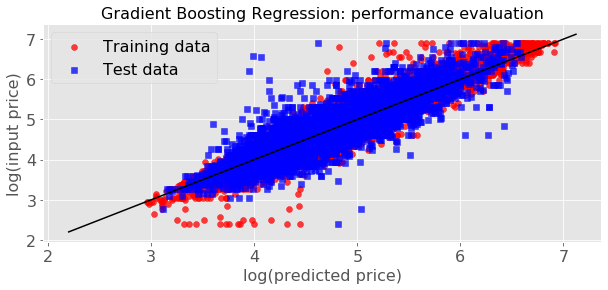
Figure 9 below depictis a scatter plot of the predicted price versus the input price for both the training and test data sets. The deviations in the test data can be observed (as evidenced by the relatively larger RMSE in table 2).

Figure 9: Scatter plot of input price versus predicted price for the gradient boosting regression (GBR) model.
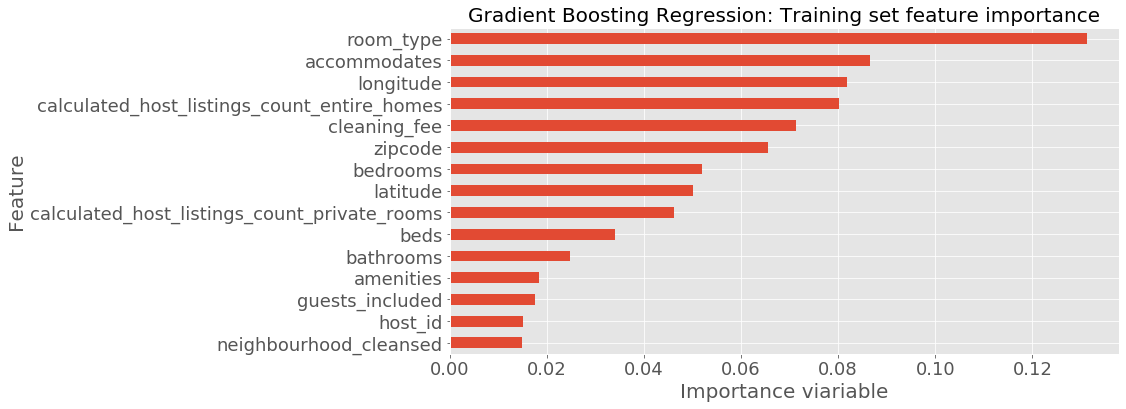
Figure 10 depicts the feature importance plot. By definition, the importance of a feature is the increase a model's prediction after the feature's values are permuted. In other words, a feature is important if shuffling its values increases the model error, while a feature is unimportant if shuffling its values leaves the model error unchanged.
Clearly the room_type categorical feature (entire home/apt, private room or shared room) and the accmmodates numerical feature (the number of guests the rental can accommodate) are the features of the highest importance. The longitude numerical feature (related to the geographical location of a rental) is the third most important feature.
V. Summary
In this study, we explored and modeled Airbnb listings data in NYC from August 2018 to August 2019. About 80% of the listings are apartments, with an average nightly price of $180. As expected, the most frequently listed amenity is WiFi internet.
Machine learning model of listing price per month based on 50 features indicated that tree based models, namely random forest regression, gradient boosting regression, and extreme gradient boosting regression, explain the price variation in the training data set quite well (as measured by the coefficient variation R2). The R2 measure for the test data set was fairly strong (about 0.8), with a root mean square error of about $60. The room_type feature was feature of the highest importance.
The study may be improved as follows: (i) expand or shrink the feature set such that RMSE error will be reduced; (ii) employ other machine learning models such as k-nearest neighbors and support vector machines.
Appendix A:
Appendix B: The Python code and data can found on github: https://github.com/rattafynn/Capstone


