Data Science Involved in PCA and Facial Images
The skills we demoed here can be learned through taking Data Science with Machine Learning bootcamp with NYC Data Science Academy.
Data Science Involved in PCA and Facial Images
Principal component analysis (PCA) is a useful tool in data analysis, especially when the number of features is large but they are also highly correlated. In short, the idea is to replace the original set of features by some of their combinations -- known as principal components -- that capture the most prominent variations in the data. One complaint about PCA is that the principal components can be difficult to interpret. Facial image analysis, however, provides a nice illustration of the idea and power of PCA whose results that can be visualized and intuitively interpreted.
The dataset
Labelled Faces in the Wild is a large database of facial images. For simplicity, I chose to use a cropped version of the images, each of which is composed of 64 by 64 (i.e. 4096) grayscale pixels. These pixels are the original set of features, but they must be highly correlated. (A random collection of 4096 pixels would almost never look like a human face!)
Principal component analysis
The distribution of the facial images can be largely captured by (i) their center, together with (ii) their most prominent variations from the center. In practice, I obtained these only from a sample of 500 images from the database, due to the limited amount of memory in my laptop.
library(pixmap)
numSamples = 500

# Import image files as pixel vectors
# (source: http://conradsanderson.id.au/lfwcrop/)
set.seed(1)
path = "data/faces/"
flist <- sample(list.files(path), numSamples, replace=F)
  # only a subset of images used due to memory limitation!
pix <- matrix(0, numSamples, 4096)
for (i in 1:numSamples){
  fname <- paste0(path, flist[i])
  pix[i,] <- as.vector(getChannels(read.pnm(fname)))
}

# Find (i) the mean pixel vector and (ii) the PCs of the re-centered pixel
# vectors responsible for 99% of the variations.
pix_mean <- colMeans(pix)
pix_mean_rep <- matrix(1, numSamples, 1) %*% matrix(pix_mean, nrow=1)
pix_ctr <- pix - pix_mean_rep
pix_eig <- eigen(t(pix_ctr) %*% pix_ctr)
numPCs = min(which(cumsum(pix_eig$values) / sum(pix_eig$values) > 0.99))
pix_PCs <- (pix_eig$vectors)[,1:numPCs]

# Save the mean and principal components
df <- data.frame(cbind(pix_mean, pix_PCs))
colnames(df) <- c("mean", paste0("PC", 1:numPCs))
write.csv(df, "PCs.csv", row.names=FALSE)
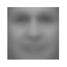
The center of the images (regarded as vectors of pixels) is best represented by their mean, which may be thought of as the "average face".
The most prominent variations in the images are given by some of their principal components. As it turns out, the first 121 principal components already manage to account for 95% of the variations, and the first 269 already account for 99%. Notice that the first principal component is quite uniform across all the pixels, meaning that the single largest varying factor in the images is simply the overall brightness. Once this factor is disregarded, we start to see more and more features of a human face.
Compression of facial images
Rather than the 4096 pixels, we can instead represent each facial image by its first 269 principal components. This is a more economic way to store these images, with only a minimal loss of information.
library(pixmap)

# Load the mean and PCs of the pixel vectors from the dataset.
mean_PCs <- read.csv("PCs.csv")
mean <- mean_PCs[,1]
PCs <- mean_PCs[,-1]

# Extract the desired principal components of all image files.
flist <- list.files("data/faces/")
for (f in flist){
  pix <- as.vector(getChannels(read.pnm(paste0("data/faces/", f))))
  pix_cmp <- round(t(PCs) %*% (pix - mean), 3)
  f_cmp <- sub(".pgm", ".csv", f)
  write.csv(pix_cmp, paste0("data/faces_cmp/", f_cmp), row.names=FALSE)
}
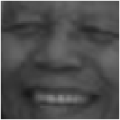
Here are some examples of facial images and their compressed versions.
Detection of facial images
For an arbitrary image, we can also extract from it the same 269 principal components and measure how much information they retain. This provides a (crude) way to automatically assess how likely the image contains a human face.
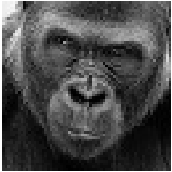
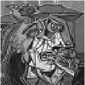
For example, in the case of the following images, the proportions of information retained are respectively 51.9%, 87.0%, 97.0%, 75.2% and 97.2%, reflecting quite well how close each image is to a human face.


