Data Study on The Zillow Zestimate Kaggle Competition

The skills the author demoed here can be learned through taking Data Science with Machine Learning bootcamp with NYC Data Science Academy.

1. INTRODUCTION

Zillow is an online real estate database with data on homes across the United States. Data shows one of Zillow’s most popular features is a proprietary property value prediction algorithm: the Zestimate.  As one might imagine, Zillow is constantly trying to improve its Zestimate.  To help advance its accuracy even further,  it launched a Kaggle competition with a $1.2 million prize.  (Feel free to check our codes at Github.)

Objective

The objective of the Kaggle competition is to predict the logerror between the predicted log error and the actual log error. The log error is defined as:

logerror=log(Zestimate)−log(SalePrice)

In plain English, the goal of the competition is to predict the difference between the Zestimate and the actual sales price of homes. This may help Zillow identify where their algorithm falls short.

Data

Kaggle provided real estate data from three counties in and around Los Angeles, CA.  Each observation had 56 features; no additional features from outside data sources were allowed in the analysis.  The data was split into two files: a training set with the actual logerror and feature information for 90,725 properties and a prediction set with only the feature information for 2,985,217 properties.  Submissions were scored based on the mean absolute error across all predictions.

Workflow

Since we had only two weeks to complete the project, we implemented a workflow with four major components: exploratory data analysis (EDA), handling missingness, feature engineering, and modeling.  As shown below, we repeated the process to improve our model until the project deadline.

As illustrated above, the process was iterated, tuned and recycled until the project deadline when final submissions were due.

2. EDA

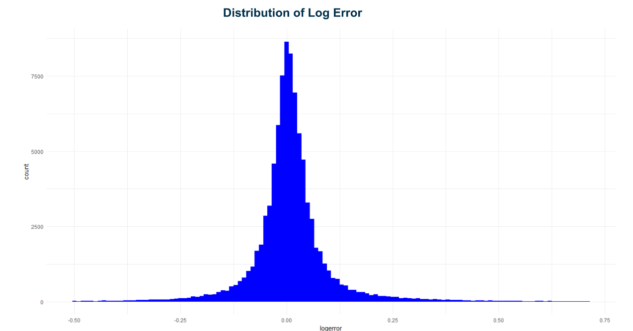
We began by exploring the training and test data to gain more insight into the overall task. As we were predicting log error and training our models on a subset of data, we first wanted to ensure that the data was normally distributed. This is an important step for maintaining the consistent distribution and performance. If we randomly split our training data into a training and test set, the model can perform differently on our test data if we do not have the same type of distribution.

There is a Gaussian (normal) distribution to the log error; this means that the random sample we use to test our model will have the same distribution as our overall data, and we can guard against overfitting.

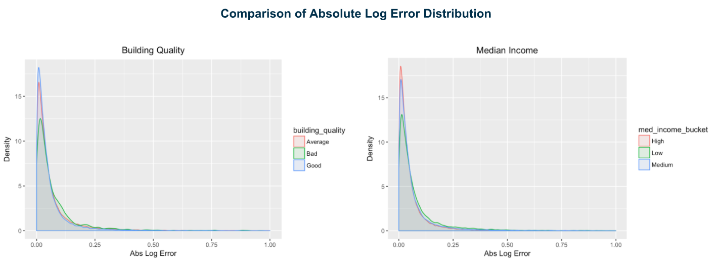
In order to begin to understand which of the 56 features were useful for our models, we looked at the absolute log error in relation to some categorical variables. For example, we can see that the absolute log error distribution is closer to 0 for higher quality buildings.

Visualizing Data Using Latitude and Longitude

We also visualized the data using latitude and longitude to identify any additional features that might help us predict the error more accurately.

In the visualization above, pockets of newer homes are highlighted. Looking at the log error (transformed for the purposes of this graph), we can see that Zillow does a better job of predicting the actual sale price for newer homes.

Training Data vs Prediction Data

One of the major pitfalls of building a predictive model is overfitting. A model that has been overfitted will perform well on training data but fail to accurately predict new observations. In order to address this, we compared the training data to the prediction data.

Overall, the distributions of the training and test data (full properties set) were similar. There were some slight differences which may have impacted the accuracy of our models.

Given the total number of features, we looked at the correlation of numerical features with both the absolute log error and each other to identify variables that might be particularly helpful in prediction.

While we did not find any numerical variables strongly correlated to the absolute log error, we did identify groups of correlated features.

We also used Principal Component Analysis (PCA), to find groups of related variables. The PCA biplot (shown above) groups correlated variables. The closer the features are to one another, the more positively correlated they are. Features across from each other are negatively correlated. As expected, PCA grouped the tax variables and variables indicating home size (e.g., bedroom count, bathroom count) together.  These analyses helped us understand the relationships between features in our data set.

3. DATA PREPARATION  

Both the training and test data had a large number of missing values that required or attention. In the training data alone, 17 variables had over 90% missingness.

Imputation Strategy

In the base case, we utilized three imputation techniques. First, we identified several binary variables and imputed with 0 and 1. Second, we imputed continuous numerical variables using the mean and discrete numerical variables using the mode. Next, for variables with a larger percentage of missingness, we imputed randomly, using a weighted distribution of observed values in an attempt to maintain the original distribution.

Feature Selection & Engineering

Following imputation, we dropped variables based on three principles: extreme missingness, duplication, and zero variance. Variables with over 90% missingness and no feasible way to determine the correct value were dropped. If variables captured the same information, such as FIPS (Federal Information Processing Standard code) and Zip Code, we only kept one. Finally, variables with the same value across all observations were dropped as they would have had no impact on our model.

We also created new variables based on our findings from PCA, including Total Room Count (bedrooms + bathrooms), Age of Home (2017 - year built), and Value Ratio (parcel tax ÷ property tax).

4. MODELING

Linear Regression

We began by fitting a multiple linear regression model to our data to better understand how our features related to each other and impacted log error. As with any line, the regression line is described by an equation that relates the predictor and response variables by assigning coefficients to the predictor variables.  The coefficient is the “influence” of the predictor on the response, holding all other predictor variables constant. The equation for the regression line is the predictive “model.”  In the equation below, the 𝜷 are the coefficients, the “xi” are the predictor variables and the “yi” is the prediction.

Fitting a linear model requires a number of assumptions: homoscedasticity of residuals, independence of errors, linearity, normally distributed residuals and independence of predictor variables. Our model violated most of these assumptions, but we proceeded for the sake of exploration. We tried some standard transformations (e.g., Box Cox) to address these violations, but they did not yield better results.

We used all 25 features to train the initial linear model, which yielded poor results (an Adjusted R2 value of 0.002422.  The Adjusted R2 value measures the effectiveness of the model with respect to variance in the residuals. Next, we reduced the model complexity using several different methods: removal of features with high (> 5) variance inflation factors (VIFs), a stepwise feature reduction using both AIC and BIC values, a Ridge analysis, and a Lasso analysis.  See Ridge analysis results in the figure below:

As anticipated, model effectiveness with regards to Adjusted R^2 did not improve by much, but it was interesting to see the significant predictors across the different methods.  

Tree-Based Modeling

The other models we used for this project fell into the regression tree-based category. Tree-based modeling is based on a structure in which the data is partitioned repeatedly at each “decision node” to minimize the residual sum of squares (RSS), or the distance of each point to the average of that group in the partition.

Tree-based algorithms implement a recursive binary splitting approach to “grow” the tree that is both “top-down” and “greedy.”  “Top-down” means that the data set is split into binary components successively starting with one, initial node.  “Greedy” means that splits at each node are based on the option with the best possible outcome at that node, not based upon a future segmentation that may lead to a better final result.  

One downfall of this approach is that it may lead to overfitting. In the extreme case, each observation would have its own partition (aka terminal node).  In this case, the RSS would equal 0, but the model would perform poorly if required to predict a new observation that is not in the data set.  

Bagging (Bootstrap Aggregation)

Bootstrap Aggregation (aka “Bagging”) is a method to mitigate against over-fitting by simulating a larger training data set to reduce overall variance. Bootstrapping takes a sample of observations with replacement from the training set to create a new data set with an equal number of observations. To estimate the testing error of a bagged model, the model predicts the response for “out of bag” observations that were not used to grow the tree.  The results are then averaged to calculate the out of bag error.

Random Forest

Random forest is an ensembling, tree-based modeling technique that uses bootstrapped training sets to build a “forest” of decision trees. Random forest helps decrease correlation and reduce model variance by randomly selecting a subset of predictors to analyze at each node of the decision tree.  Overfitting is unlikely due to the random, de-correlated nature of the tree building process.

Gradient Boosting Machines (GBM)

GBM builds trees sequentially using the residuals from the previous trees to build the next tree.  Given a decision tree model, we fit a new tree to the residuals of the current tree. The new decision tree (based on the residuals) is then added to the current decision tree, and the residuals are updated.  To combat overfitting, the tree depth (number of splits away from the initial node) is limited, and a learning rate (shrinkage rate) is introduced.

Cross-Validation and Hyperparameter Tuning

For all models, K-fold cross-validation was performed in order to prevent overfitting and search for the optimal hyperparameter settings over a tuning grid.  K-fold cross-validation involves splitting the data into K folds, setting one fold aside, training a model with the other folds and testing with the fold that was set aside. The results are then averaged together for a single estimation with reduced variance. Due to time and computing power limitations, we limited our analyses to 5 and 10-fold cross-validation.

We also partitioned 25% of our training data and held it out for testing before we trained a full model with all training data.  This helped us quickly assess model performance without predicting log error for 2,985,217 observations and submitting our prediction to Kaggle for feedback.  

Hyperparameter Tuning

Hyperparameters are the “higher-level” model properties that have an effect on the model training process (e.g., learning/shrinkage rate, tree depth).  Our team used a grid search to obtain optimal hyperparameter settings for all models considered. Conceptually, a grid search iterates a model through a hyperparameter grid to find the combination of hyperparameters that minimizes the loss function (or maximizes the objective function, i.e. ROC). We also used a random search for optimal hyperparameters, but the results were similar and  the random search took much longer than the standard grid search.  

With more time, we would have attempted a Bayesian Optimization hyperparameter strategy since research suggests that this technique yields better results while expending less computational power and taking less time. Bayesian Optimization retains information from previously sampled points when searching for the global minimum/maximum of the objective function.  

Initial Results

GBM yielded the best results from our initial round of modeling. See the table below for the hyperparameters selected and results for the 3 model types:

5. MODEL ITERATION

We treated the results from our first round of modeling as a baseline and returned to the beginning of our workflow to try to improve our models. We implemented several strategies independently to see how they would affect our results.

Additional Strategies

• Trimming Features by Importance: In order to reduce model complexity, we aggregated the most important features from each of our best initial model runs and chose 11 features to test.  Reducing model complexity actually reduced the accuracy of our models.

• Additional Feature Engineering: We created additional features based on the most important features in our initial models.  For example, we created a metric to represent the ratio of the home’s structure tax to its land tax.  Some of these features improved the accuracy of our predictions and were used in predicting our final submission for log error.  

• Adding External Features: Although not formally allowed by the Kaggle competition rules, we wanted to see if adding external features would help predict logerror. We incorporated several variables from the Census Bureau's 2015 American Community Survey, including median income, population, and monthly housing costs.  Unfortunately, adding these features did not improve our results.

• Re-Imputation: In our second attempt, we used a “simpler” imputation strategy. Features that were originally imputed with a random weighted sample were instead imputed with either the mean or mode. This method did improve our results.
• Handling of Outliers: Several features in our data set had outliers (observations greater than 3 standard deviations from the mean). We suspected these outliers might be affecting our model performance and tried a few strategies to replace them, including replacing them with the median and complete removal.  All of these strategies decreased the predictive power of our models.

Ensemble Learning:

Ensemble learning is used in machine learning because the generalization ability (predictive power) of an ensemble is greater than a single “learner” (model). For the best results, correlation between learners should be minimized - where one model is deficient, another might excel.  Ensemble learning did not improve our results, likely due to high model correlation.

Final Results

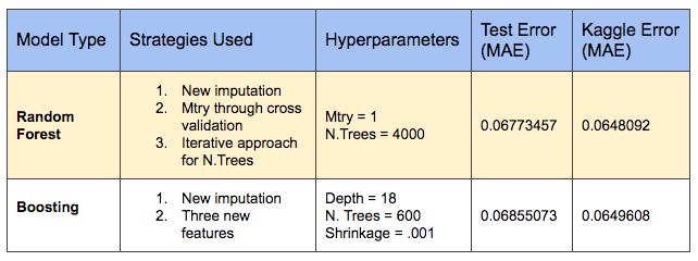
Our Random Forest model produced the lowest logerror across all models we tried. Surprisingly, a grid search for the optimal mtry (the number of randomly selected features that are analyzed at each decision node) returned a value of 1. Since several of our features were correlated, selecting only one feature at each node might produce the least correlated trees. The final model run results are captured in the table below:

6. SUMMARY AND CONCLUSIONS

Given the amount of missing data and relatively large number of features in this project, imputation strategy and feature engineering were very important with respect to reducing prediction error. Using a simple imputation strategy was the most significant factor to improving our results.

With more time, we would continue to iterate on our workflow and introduce new strategies to improve our model results.  There were several modeling techniques that the team did not have a chance to explore due to time constraints, including Neural Networks and Support Vector Regression. Given the importance of choosing the right imputation method, we would attempt methods that require more time and computational power, such as KNN.