Evaluating Home Buying Opportunities
Which combination of housing features has the greatest impact on sale price? Using machine learning techniques to predict the sale prices of homes in Ames, Iowa, Evaluating Home Buying Opportunities with Machine Learning is a tool for home buyers and sellers to guide their value-based investment decisions. This predictive model (RMSE of 0.119) scored Top 16% among 5,000+ other models in a Kaggle competition (as of March 2020), combining advanced techniques without sacrificing interpretability.
|
Authors: Richard Choi, Marek Kwasnica, You-Sun Nam |
Table of Contents
- Introduction
- Dataset and Model Evaluation
- Data Cleaning
- Model Selection and Performance
- Feature Selection
- Conclusion
- Contact
Introduction
Purchasing a home is one of the most life-changing decisions that any person can make. Whether it is to procure a home for your family, invest in a high-returning asset, or to do a bit of both, it is pivotal that a prospective home buyer makes this purchase at the correct price. Determining the appropriate value of a home, however, can be a significant challenge due to the fact that the valuation of a home is dependent on a seemingly endless number of features that a home can possess.
To address this challenge, this project endeavors to implement machine learning techniques to predict the sales price of houses in Ames, Iowa.
Dataset and Model Evaluation
The dataset used for this exercise comes from the House Prices: Advanced Regression Techniques, Kaggle competition archive, and features 79 categories of features concerning 3000 homes in Ames, Iowa. The set includes 43 categorical (eg. type of finish, zoning) and 36 continuous features ( eg. lot square footage, number of rooms). The choice of machine learning model must be sensitive to the relationship between both types of information and the target variable: sale price.
The performance of the machine learning models in this project will be evaluated by comparing the predicted home values with the actual sales price. The metric through which we measure this will be the Root Mean Squared Error (RMSE).
Data Cleaning
Before training our models, it is pivotal to examine our data and transform them in a manner that is suitable for our predictive models.
Observing Sales Price
To begin, we examined the distribution of our target variable, the sale price of homes, by plotting the number of homes at each price (Figure 1.1). We can see that Sale Price is positively (or right) skewed with most of the home prices landing the $100k to $200k range, but a large range of possible prices above $200k (while no houses can sell for below $0).
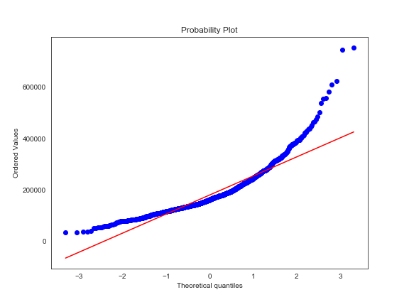
This indicates that our Sale Price is not normally distributed, and we can expect that some predictive models, such as linear regression, may have some limitations with respect to the assumption of normality at the extremes of the price range. We created a Q-Q plot, splitting the price range into quantiles and plotting them against an idealized normal distribution of prices, a Q-Q plot (Figure 1.2), to further confirm the suspicion that the data is not normally distributed.
We can address this issue by applying a logarithmic transformation that will make the distribution of Sale Price more fit for training our models as we can confirm with the histogram and Q-Q plots seen in Figures 2.1 and 2.2, that we see after applying this transformation.
Addressing Outliers
Having normalized our target, we next examine all other features for interdependence and outliers. The two salient features that helped in identifying outliers in this exercise are General Living Area and Total Basement Square Footage.
General Living Area
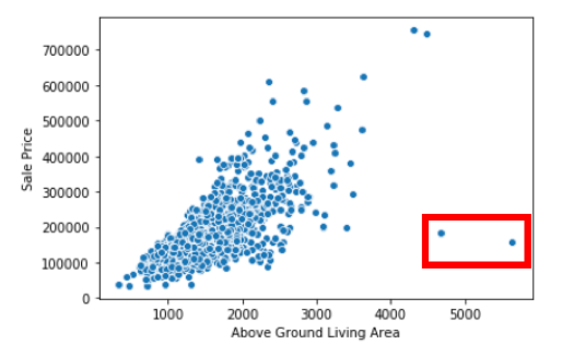
Here in Figure 3.1, we see two observations with substantial living areas that have sale prices that are not consistent with what we would expect.
When we remove these outliers, the linear relationship between Sale Price and General Living Area is a little clearer (Figure 3.2).
Total Basement Square Footage
On a similar note, we see homes with significantly larger basements, which do not seem to be in line with the otherwise linear relationship between basement size and sale price seen in Figure 4.1.
Removing this outlier allows us to more easily see the relationship between the variables in Figure 4.2.
Missing Data and Imputation
The next step in preparing our data lies in accounting for missing data. There are 30 features in this data set — all but 6 of them have less than 5% of observations missing as shown below in Figure 5.1:
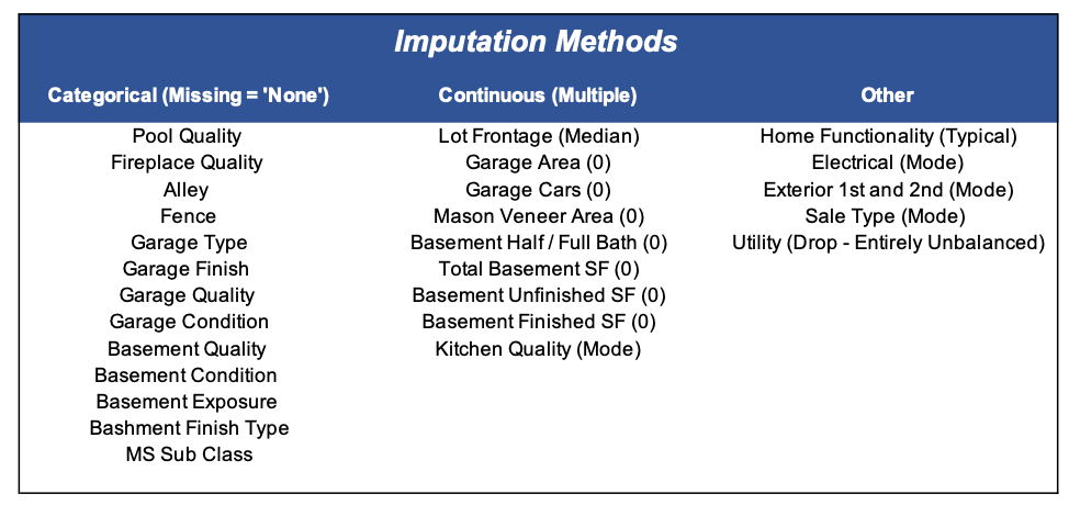
To remedy this issue, we must impute missing values or drop features with too many non-imputable missing values. The type of missingness and imputation methods used to impute data for the features in this dataset are broadly e described and summarized below:
- Categorical variables: missingness usually implies the absence of the variable, imputed as 0.
- Continuous variables: missingness typically implies 0, but in some circumstances, mean, or mode is used depending on the inherent distribution of the variable
Model Selection and Performance
Model Selection
To explore how housing features impact sale price , we trained several linear and non-linear models.
We began with linear regression, which was used as a baseline model to measure the performance of machine learning models. While the baseline model was acceptably accurate in the central range of $100k-200k, as mentioned before, it did not predict accurately if a house’s real sale price was on the extremes of the price range scale.
Next, more advanced variants of multiple linear regression — Lasso, Ridge, and ElasticNet models — were used to predict sales price. These variants have additional constraints to reduce variance by adding a different regularization term called lambda which penalizes model complexity. Each model employs a different lambda, differentiated as lambda_1 (L_1) and lambda_2 (L_2), to reduce model complexity. L_1 regularization in Lasso has the additional benefit of performing feature selection.
|
TECHNICAL NOTE Ridge regression via L_2 regularization and Lasso regression via L_1 regularization use different penalty terms, resulting in Ridge keeping all model features and Lasso reducing the number of features. This is because unlike L_2 regularization in Ridge which shrinks feature coefficients towards (but never reaches) zero, L_1 regularization in Lasso actually converts some feature coefficients — mainly, those responsible for large variance — to zero. ElasticNet combines both approaches of Ridge and Lasso, and attempts to balance them for the optimal solution. |
Following linear regression models, we explored nonlinear machine learning models, Random Forest and XGBoost. The purpose of this was two-fold; firstly we wanted to confirm if the nonlinear models outperform linear models, and secondly, we wanted to see which features had the most impact on sales price, thereby reducing predictor features.
|
TECHNICAL NOTE Random Forest and XGBoost are both ensemble learners of decision trees, which iteratively split the data into subsets depicting different outcomes from a set of decisions, with key differences. (Ensembling is a machine learning technique which trains multiple models — also known as “[weak] learners” — using the same algorithm.) Random Forest uses a variation of “bagging,” which builds n (number of) learners in a parallel fashion using random sampling with replacement. XGBoost, on the other hand, uses “extreme gradient boosting ,” which, in turn, is a variant of boosting. Boosting sequentially builds an n (number of) learners using random sampling with replacement over weighted data. |
Model Performance
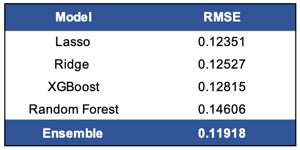
In exploring these techniques, we found that lasso was slightly more accurate than ridge, and ElasticNet would essentially become a lasso regression. While neither XGBoost nor Random Forest proved to be more accurate than linear regression models in predicting sales price, these models were useful in narrowing down which features were most influential on sales price. (In this analysis, we focus on Random Forest’s drop-column importance.)
In conclusion, we find that Lasso Regression is the most effective model on a standalone basis: RMSE of 0.124 (Figure 6.1). However, as there are merits to the different methodologies for different purposes (such as capturing nonlinear relationships or decorrelating data), the best method overall in terms of predictive accuracy, is to ensemble the methodologies with equal weight: RMSE of 0.119 (Figure 6.1).
Feature Selection
Feature Importance
When we use Lasso Regression to conduct feature selection, we see that the important variables that can be leveraged to generate home value are:
Overall QualityGeneral Living AreaTotal BathroomsGarage Car CapacityBasement Square Footage
Another method that can be used is drop-column feature importance through random forest. Drop-column feature importance compares the performance score of a reduced model (i.e. a model with a dropped feature) to the performance score of the baseline model with all features. Each feature is then ranked based on the difference of the performance, where higher difference means more important.
We get a different ranking of top 5 key features through random forest’s drop-column feature importance method from those selected by lasso regression’s regularization process:
General Living AreaNeighborhoodOverall QualityYear RemodeledLot Area
What accounts for the different rankings? Simply put, regularization and drop-column importance are different methods. Lasso regularization provides a continuous decrease in the importance of the feature by varying the (L_1) penalization of the linear regression, where the last one that goes to zero is the most important and so on. Random forest drop-column importance removes a column from an ensemble of regression tree models to measure its effect on prediction.
Since General Living Area and Overall Quality appeared in both methods, we have stronger evidence that they have a greater impact on sale price than the other features.
Feature Dependence
Feature dependence through Random Forest is a useful way to determine which features are redundant to include in the predictive model with respect to tree based models. Removing them can increase model performance by decreasing variance. This approach identifies features that are dependent on other predictor features by training a model to use a predictor feature as the new target feature and use the remaining features as predictors. The output is R2 prediction error (how predictable the target feature is using predictor features); the higher the score, the greater the dependence on other features.
| Feature | R2 prediction error |
General Living Area |
0.973093 |
2nd Floor Square Footage |
0.957733 |
Building Class |
0.946657 |
Year Built |
0.93752 |
1st Floor Square Footage |
0.913189 |
As we can see, General Living Area tops the list with the greatest dependence score. This isn’t entirely surprising, given that General Living Area is simply the sum of the first floor area, the second floor area, and the basement area in square footage. To confirm, let’s take a look at which features are important in predicting General Living Area and other select features.
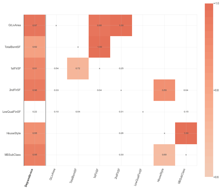
Figure 8.2 Feature dependence of select features, displayed as a matrix
From the above matrix, we can see that 1st Floor Square Footage is important in predicting Total Basement Square Footage and General Living Area. Likewise, 2nd Floor Square Footage is important in predicting General Living Are. Normally, this would mean we can drop General Living Area from the model and keep each floor feature.
But depending on the question being asked, we can keep General Living Area (which is the total area of all floors) and drop 1st Floor Square Footage, 2nd Floor Square Footage, and Total Basement Square Footage instead. That is, if you’re interested in figuring out which floor has the greater impact on sales price, then it would make sense to drop General Living Area given the feature dependence. But if you’re comparing the area of a home to a broad, diverse range of factors unrelated to area, then it would make sense to keep General Living Area and drop the individual floor features. In our case, we’re more interested in gaining a macro level of insight, which means we would keep General Living Area and drop the individual floor features if we were to rerun the model with reduced features.
Conclusion
In conclusion, when leveraging machine learning techniques to make an informed home purchasing decision, it is best to ensemble different machine learning models, all with their own merits, to extrapolate a valuation. That said, once a home is purchased and avenues to improve home value are being considered, we humbly offer the following recommendations to generate value:
- Improve
Overall Quality,such as upgrade the material and finish of the home - Expand
General Living Areain the home, such as build a new wing
Contact
If you have any questions or comments, please feel free to reach out to any of us on LinkedIn or GitHub.
Meet Our Team
Contact our team (NOTE: names are listed in alphabetical order of surname):
- Richard Choi: LinkedIn | GitHub | Blog
- Marek Kwasnica: LinkedIn | GitHub | Blog
- You-Sun Nam: LinkedIn | GitHub | Portfolio | Blog
- Ivan Passoni: LinkedIn | GitHub
If you'd like to check out our other work, please see our other blog posts and individual portfolios!


