House Prices: Advanced Regression Techniques
Introduction
For most people, buying a house is the single largest investment decision they will make. Prospective buyers typically require years of saving to generate a down payment and are then committed to making monthly mortgage payments over a thirty year period. Moreover, taxes, insurance, electricity, heating, cooling, and home maintenance are additional costs associated with home ownership. For potential buyers, it's advantageous to know where house value may be derived from and what a prospective house is worth. Similarly, existing homeowners looking to sell and maximize investment would benefit greatly in their decision-making process if they can predict the price of their home prior to listing it.
The project explores advanced regression techniques to predict housing prices in Ames Iowa. The Ames Housing dataset was compiled for use in data science education and can be found on Kaggle. The data includes 79 features describing 1460 homes. While house price prediction is the main focus, the authors also aim to answer the following questions:
What features are most correlated with housings prices?
What features are least correlated with housing price?
How does the feature engineering impact model performance?
Which machine learning models perform best predicting price?
Various imputation methods are employed to address missingness. Transformation and standardization are used to increase model performance. 5-Fold cross-validation is used to tune Hyper-Parameters on various models.
All machine learning methods are applied in Python using scikit-learn package. R is used for supplemental statistical analysis and visualization.
Data can be found: https://www.kaggle.com/c/house-prices-advanced-regression-techniques#description
All code can be found here: https://github.com/Joseph-C-Fritch/HousingPrice_ML_Project
Initial Data Analysis
One of the first and most important steps of data analysis is to look at the data. From the count, we can already see that there are missing values in the dataset. We can also see that the difference in mean and standard deviation across variables is quite large.
Next, we take a look at variables with high skew and kurtosis, which can distort the results of our prediction model if the skew is not taken care of appropriately.
Missingness & Imputation
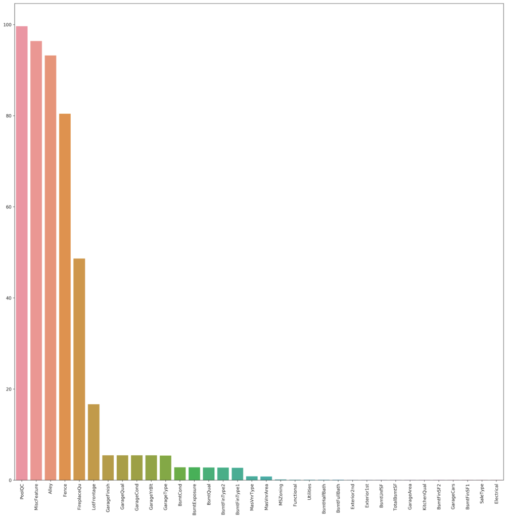
Next, we can take a look at missingness in the dataset. The PoolQC, MiscFeature, Alley, and Fence are missing in 80% of cases; FireplaceQua is missing in 49% of cases; LotFrontage is missing in 17% of cases; GarageFinish, GarageQual, GarageCond, GarageYrBlt, GarageType are missing in 5% of cases; and 23 variables are missing in less than 5% of cases.
In most cases, we were able to fill in the missing value with the NA/”0” if the feature was not available for the particular home, or with the most common value. In other cases, we took a more targeted approached and filled in values based on neighborhood, or based on existing quality and condition information (especially for Garage and Basement values).
Outliers
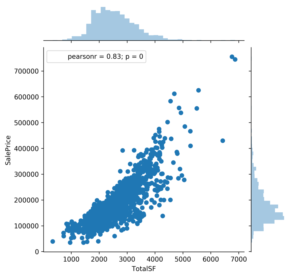
We also looked at outliers in the dataset to see for any observations that would clearly distort our model. Looking at the relationship between Total SF and Sale Price, we can see that there are two outliers, and the removal of these two observations increases the correlation of total square footage and sale price from 0.78 to 0.83.
Transformation and Standardization
Among the numerical features, we chose to transform LotFrontage, TotalSF, and SalePrice, either log or Box-Cox transformations. Here, we can clearly see that our target variable, Sale Price, is heavily skewed to the right, so we can apply a simple log transformation so it follows a Gaussian distribution.
After transforming our skewed variables and removing outliers, we then standardized our numerical features, which is essential for our models to accurately determine the size and importance of regression coefficients.
Feature Engineering
Many categorical features consist of subcategories containing fewer than twenty-five observations. To avoid overfitting, sparse categorical variables are consolidated. For example, the feature MSSubClass includes sixteen subclasses with six of them containing less than 25 observations. A histogram of MSSubClass is illustrated below. These sparse categories are combined into a single sub-class referred to as “other”. A similar procedure is conducted on other categoricals features that meet the defined sparse criteria.
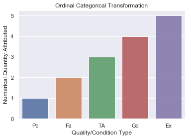
Ten categorical features describe quality and condition ratings for the various house attributes. For example, basement quality and condition are represented with a rating of either poor, fair, average, good or excellent. Such ordinal categorical variables are quantified with a score from one to five retaining their order and avoiding dummification. A graphical representation of this relationship is illustrated below.
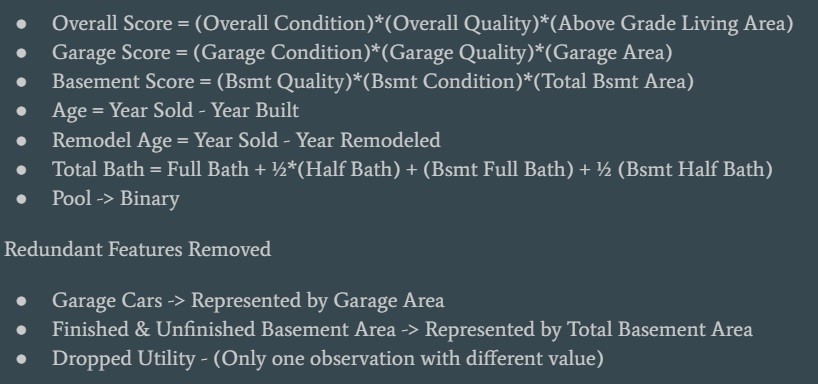
To increase predictor strength while simultaneously reducing complexity and multicollinearity, interaction features are introduced. A scoring system is developed which combines quality and condition ratings with square footage. For instance, basement quality, basement condition, and total basement square footage are multiplied together to create a new feature basement score. A similar procedure is carried out on the exterior, garage, kitchen and overall features. A summary of notable interaction features is shown below.
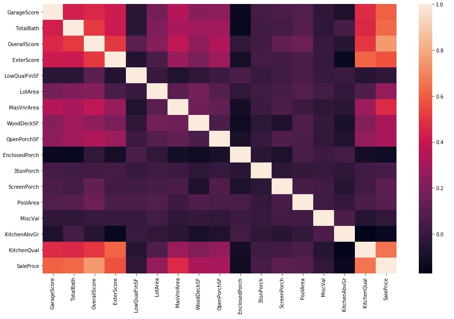
The following correlation heat maps illustrate multicollinearity and predictor strength before and after interaction feature creation. It can be seen that feature engineering has reduced multicollinearity between predictors while increasing predictor strength with the house sale price.
Modeling
Lasso
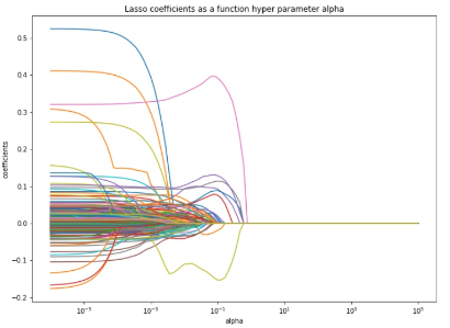
Regularized regression is explored using the Lasso method. The l1 penalty is applied and hyperparameter tuning of lambda is conducted using five-fold cross-validation. Scikit-learn’s built-in Lasso and LassoCV are used. Optimal alpha is approximately .01. The plot below illustrates beta coefficients as a function of hyperparameter alpha.
As expected, as alpha increases, many of the coefficients are forced to zero according to the l1 penalty. Feature selection is carried out by Lasso and the resulting features are shown in the bar chart above. A total of 49 features are selected and the newly created interaction features provide amplified predicting power as they constitute four of the five top coefficients by absolute magnitude. The resulting cross-validated RMSE is .13666
Elastic Net
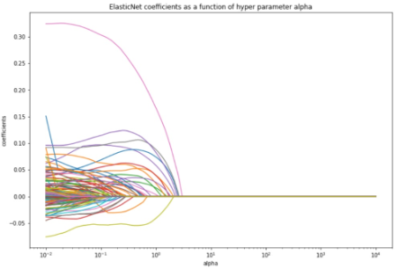
Regularized regression is explored using the Elastic Net method. The l1 and l2 penalties are applied and hyperparameter tuning of lambda and rho are conducted using five-fold cross-validation. Scikit-learn’s built-in ElasticNet and ElasticNetCV are used. Optimal alpha is approximately 0.026 and optimal rho is 0.25 The plot below illustrates beta coefficients as a function of hyperparameter alpha.
As alpha increases, some of the coefficients are forced to zero according to the l1 penalty but many more only attempt to converge to zero given the l2 penalty. Therefore more features are selected in the process. The top twenty resulting features are shown in the bar chart above. A total of 71 features are selected and the newly created interaction features again provide amplified predicting power as they constitute four of the five top coefficients by absolute magnitude. The resulting cross-validated RMSE is 0.13904.
Extreme Gradient Boosting
Extreme Gradient Boosting is used as an alternative tree-based modeling method. A grid search is used to perform five-fold cross-validation to tune multiple hyperparameters. XGBoost and Scikit- learn’s built-in GridSearchCV are used. Optimal tuning parameters are highlighted below. The plot below illustrates beta coefficients as a function of hyperparameter alpha.
The top twenty features of importance are shown in the bar chart above. The features selected are slightly different from those selected in Lasso and Elastic Net but again the newly created interaction features provide amplified predicting power as they constitute four of the six top features of importance. The resulting cross-validated RMSE is 0.13336.
Feature Engineering - Modifications
A second iteration of feature engineering is conducted. There are heavy correlations between Garage Area and Garage Cars and between 1stFlrSF and TotalBsmtSF. We can combine aspects of these features in order to reduce some multicollinearity and create features with a higher correlation with Sale Price without losing any information. The scoring system used previously is removed and sparse categorical variables are not reduced.
To reduce some of this multicollinearity, we reduced our square footage information into one variable, TotalSF, by combining 1stFlrSF, 2ndFlrSF, TotalBsmtSF. Similarly, the number of bathrooms are combined into one variable, Bath. All porch square footage is summed into one variable, PorchSF. GarageArea and GarageCars are multiplied together to make one variable that had a stronger correlation with Sale Price.
After combining correlated features together, filling in missing values, transformation, and standardization, we can see that the multicollinearity is decreased among numerical variables, but correlation with Sale Price remains high.
Ridge Regression
Ridge regression is another form of regularized regression (https://www.statisticshowto.datasciencecentral.com/regularizatio /) that utilizes a penalty term to reduce complexity of a model. The L2 regularization term adds a penalty that is equal to the sum of the squares of the beta coefficients, thereby forcing the coefficients to shrink towards zero. While the coefficients are not actually forced to zero, ridge regression helps to combat the issue of multicollinearity (http://www.stat.cmu.edu/~larry/=stat401/lecture 17.pdf) between different features (which may result in inaccurate estimates and increased standard errors of coefficients) by reducing the variance of the model (although increasing the bias).
To optimize the hyperparameter alpha (or lambda, depending on the terminology), we used a five-fold cross-validation scheme within the range 1e-6 to 1e6, which returned an optimal value of 18.73, and our best Kaggle RMSE with ridge regression alone was 0.12112.
We can see that our residuals are normally distributed, but there are some clear outliers that can be removed. However, removal of these outliers tended to result in a worse Kaggle RMSE, which indicates that there is pertinent information in at least some of these observations that should not be removed.
We can see that our ridge regression model performs quite well on our training data, and there is an overlap between actual sale price (on train data), predicted train sale data, and predicted test sale data is quite
Support Vector Regression
We also used Support Vector Regression (https://www.saedsayad.com/support_vector_machine_reg.htm) with a radial-based kernel and used five-fold cross-validation to optimize the hyperparameters epsilon, cost, and gamma. Much like any other regression technique, the goal of support vector regression is to minimize the amount of error. Gamma is similar to K in K-nearest-neighbors, with a small value of gamma taking global information into account, and a large value of gamma taking local information into account. The cost parameter is similar to lambda in the previously-mentioned Ridge, Lasso, and Elastic Net models and dictates the influence or size of the error term. The epsilon parameter controls the epsilon-insensitive region, which defines the margin of tolerance where there is no penalty associated with observations within the region. Hyperparameter optimization gave an optimal epsilon of 0.1, cost of 10, and gamma of 0.001, resulting in a Kaggle score of 0.12079.
Gradient Boosting Regression
Gradient Boosting Regression is an ensemble model which builds successive decision trees. While each individual tree is a weak learner (does not perform well on test sets), successive trees attempt to correct for these shortcomings by fitting to the residuals of the previous tree. Using five-fold cross-validation and a learning rate of 0.05, we found our optimal number of estimators to be 2000 (total number of boosting stages) and our optimal depth of each tree to be 2 (2 nodes), giving a Kaggle score of 0.12348.
Gradient boosting regression selected 152 features to be important in the prediction model, with TotalSF, KitchenQual, OveralQual, and Baths (unsurprisingly) being selected as some of the top features.
Conclusion
Finally, we generated a model based on the average prediction (https://en.wikipedia.org/wiki/Ensemble_averaging_(machine_learn ing)) of Ridge, Lasso, Elastic Net, and Gradient Boosting Regression, figuring that the errors made by each individual model may be mitigated when weighted on average, and found that this model actually had the best Kaggle RMSE of 0.11973.
In general, ridge regression seemed to outperform the other models with feature engineering, while support vector regression gave us our best individual score by inputting all features without engineering.
Some ways that we can create a more accurate predictive model are (1) to carefully choose feature engineering to remove more multicollinearity and create stronger predictor variables, (2) to identify outliers and be mindful when deciding to remove them, (3) to tune more hyperparameters (i.e. testing a polynomial kernel for SVR), and (4) try stacking, ensembling, and weighing models in various ways.


