Kaggle Competition: Building Algorithm to Predict Allstate Claim Severity
1. Introduction
When a claim is made, a loss is incurred for an insurance company when the coverage is greater than the accumulated payment from the customer. Thus for these companies, it is valuable to "know" of the potential loss in advance. Allstate is currently developing automated methods of predicting the severity of car accident claims. As a result, an open competition is hosted on Kaggle.com. In this project, we are aiming to leverage our machine learning skill and build a prediction algorithm to link 130 variables to the outcome "loss", with the goal of minimizing the mean absolute error (MAE). All python and R scripts used for this project can be found here.
2. Exploratory Data Analysis
The number of observation in the training set is 188318. It has 116 categorical and 14 numerical variables, and all variables are not interpretable. Due to the high amount of features, it is necessary to perform exploratory data analysis to gain some insights of these variables.
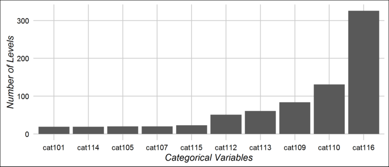
As shown above, some categorical variable has more than 100 levels, like cat110 and cat116. These features will cause trouble for building tree-based model. Thus encoding them to numeric variables are especially needed.
For 14 continuous variables, they all have values ranging from 0 to 1, meaning that some kinds of transformation is applied to each of them. Some variables are highly correlated, which will increase the coefficient variance for regression models. The outcome "loss" shows strong skewness, therefore a log transformation is applied to this column throughout the work.
3. Data Processing
Given 116 categorical variables in the dataset and some of them have more than 100 levels, huge amount computation power is needed for training the model. To make the computation doable on our PC, it is necessary to encode these categorical features to numeric columns. In this project, we decided to apply three different encoding techniques to the original data. As you will see in the later section, we apply each machine learning algorithm on every encoded version and pick out the relatively strong predictors for the future model stacking.
3.1 Encoding I
As shown in the figure above, the idea of encoding 1 is to expand the multinomial features into binomial variables, after this transformation we filter out the variables with near-zero-variance and performed one-hot encoding to the remaining columns. After encoding 1 the final data contains 193 variables in total.
3.2 Encoding II
Instead of converting to binomial, the idea of encoding 2 is to directly perform one-hot encoding on all categorical variables. However, it should be noted that before transforming to numeric, it is important to identify all unmatched values between training and testing set, and set these values to the last level in this column. After encoding 2 we have 130 variables.
3.3 Encoding III
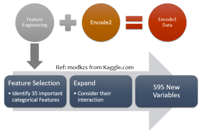
Encoding 3 is adapted from Kaggle kernel by modkzs. This method applies feature engineering to generate new variables and then perform encoding 2 to convert everything to numeric. 35 relatively important features were selected from XGBoost and Linear Regression, and the combination of any two features were generated as new columns. After pre-processing 595 new variables are created.
4. Exploratory Algorithm Selection
Since there are so many different supervised machine learning models to choose from, it is crucial to select the optimal models suited for this competition. This can be done by establishing a benchmark of viable models based on their MAE (mean absolute error). From this benchmark, we can choose the models with lowest MAEs for later process, such as experimenting different encoding method and model stacking. Ultimately, we select five distinct models to construct the baseline:
- LASSO Regression
- Ridge Regression
- Decision Tree
- Random Forest
- eXtreme Gradient Boost (XGBoost)
For this exploration, the categorical features were converted to “numerical” features via the method of one-hot encoding without any feature selection method to explore the dataset in its entirety, to ensure the viability of the generalized linear models, and to reduce computational handicap for the tree-based models.
Out of the five selected models, LASSO and Ridge regression was selected to serve as a generalization of linear regression model. Decision tree was selected because it is a suitable model for this dataset. Random Forest and XGBoost were selected because of their high accuracy and ensemble nature.
We also omitted models that we believe are not fit for this dataset, including k-Nearest Neighbor (k-NN) and Support Vector Regressor (SVR). The reason for the exclusion is that we did not feel distance-based models are viable for this dataset due to large amount of categorical features.
The minimum validation MAE is obtained through model parameter tuning. We decided to tune one critical parameter per model via 90%-10% train-test split validation. The MAE of each validation is then plotted against the tuning parameter; the models with the lowest MAEs will be ideal from the bias-variance trade-off. Since this is an exploratory analysis, a coarse estimation of MAE will be enough in distinguish models. No finer parameter tuning was necessary.
4.1 LASSO Regression
The LASSO regression was validated using the lambda parameter with ten values ranging from 100 to 0.001. The minimum MAE is 1304 with a corresponding lambda of 0.1668. This lambda represents the best lambda from the bias-variance tradeoff, a higher lambda will result in an increase in bias (underfit) while a lower lambda resulting in an increase in variance (overfit).
4.2 Ridge Regression
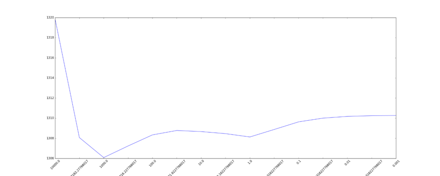
The Ridge regression was validated using the lambda parameter with fifteen values ranging from 10,000 to 0.001. The minimum MAE is 1306 with a corresponding lambda of 1000. Similar to LASSO regression, a higher lambda will result in an increase in bias while a lower lambda resulting in an increase in variance. Also the range of lambda was increase to [10000, 0.001] because of a local minimum occurring at lambda equals to 1. Since LASSO and Ridge regression are related (l1 and l2 norm), their MAEs are very close.
4.3 Decision Tree
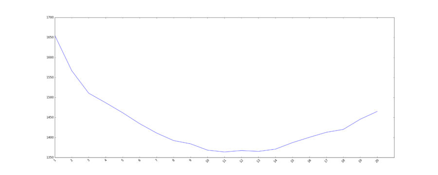
The decision tree model was validated using the tree depth parameter ranging from 1 to 20. The minimum MAE is 1364 with a tree depth of 11. The bias-variance off is also observed here. Since the decision tree tends to overfit easily, it is no surprise that the MAE is higher.
4.4 Random Forest
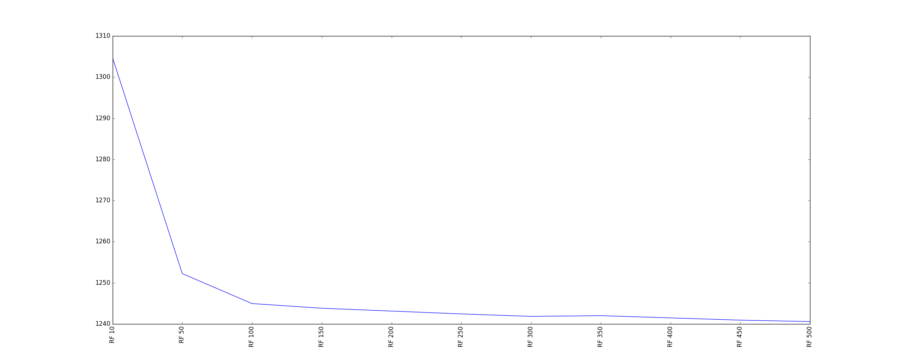
The random forest model was validated using the number of trees parameter ranging from 10 to 500. The minimum MAE approaching 1240 at max number of trees of 500. Due to the nature of random forest model being an ensemble model and its unique property of inducing randomness in observation and feature, it is practically impossible to overfit. Thus, it is nearly impossible to find a global minimum of MAE, but the MAE will eventually approach an asymptote and reach a limit.
4.5 eXtreme Gradient Boost (XGBoost)
The XGBoost model was validated using the number of boosted models parameter ranging from 10 to 1500. The minimum MAE approaching 1200 at max number of trees of 1500. Similar to random forest, XGBoost is also an ensemble model, therefore it is more robust to overfitting compared to non-ensemble models. Also, ensemble models generally perform better than non-ensemble models, which is true in this analysis, random forest and XGBoost both yield a MAE in the 1200, whereas all the non-ensemble models scored 1300 and more.
4.6 Neural Network
The neural network with three hidden layer was chosen to build the model since it significantly out-performs the one and two-layer derivatives. Cross-validation was applied during the training process. The workflow can be summarized as the following steps:
- Create dummy variables
- Generate sparse matrix
- Normalize continuous variables
- Set parameters for neural network
- Stack using 10-fold cross-validation and bagging
- Use MAE to evaluate the performance
Our final neural network model was obtained after several rounds of parameter tuning. By changing the number of nodes in each layer, number of hidden layer, and regularization method, our final model has the structure shown above. The neural network is relatively computational expensive to build. However, it shows relatively better performance than most of other algorithms we tested.
4.7 Model Summary
| Model | MAE |
| LASSO | 1304.6 |
| Ridge | 1306.0 |
| CART | 1363.9 |
| Random Forest | ~1240 |
| XGBoost | ~1200 |
| Neural Network | ~1200 |
The main objective of the exploratory model selection is to select the models with most potential for this dataset. From the summary table, we can conclude that XGBoost and Neural Network models produced the lowest MAEs, thus we selected these two models for further analysis and model stacking.
5. Model Stacking
With the strategy in mind, we started to validate each model on all three encoded dataset. At this moment, our top-3 strongest single predictors are XGBoost on encoding 2, 3, and Neural Network on original dataset. To further boost the performance, model stacking is necessary.
Above is the workflow of the model stacking. First, we randomly split the training set to two subsets. For each algorithm, two parallel models are built using different subsets. The parameters used in each training process were tuned via cross-validation. After training process, each model is used to predict the complementary data to avoid bias. Finally two predictions are bind together and used as a variable ready for building the stacking model.
Once we collect multiple predictions, a second-layer model is built using all predictions as variables. Three candidates for stacking model were examined - General Additive, Gradient Boosting and XGBoost. Among all three algorithms, Gradient Boosting generally performs better in every combination of predictors, therefore is selected as our stacking algorithm.
Figure 13. Current result (measured in MAE)
As shown above, the performance for three individual predictors shows MAE of 1114 and 1108 for two XGBoost models, and 1128 for neural network. The improvement is significant, as we were able to drop the MAE as low as 1103.82 after model stacking.
6. Milestone and Future Plan
By the time we submit the project, we were able to reach 6% on the global leaderboard. After exposure to this competition for two weeks, our findings are:
- Feature engineering is very necessary before model building.
- XGBoost and Neural Network are two algorithms that performs the best on this dataset.
- Stronger the individual predictor, better the stacking results.
Currently we keep working on more in depth feature engineering along with building more neural network models for each of the encoding method. After seeing the performance boost on the encoded dataset for every algorithm, we hope to see a increasing performance for neural network as well. By combining more strong predictors in our stacking model, hopefully we can climb higher on the leaderboard.


