Kaggle Higgs Boson Machine Learning Challenge

This blog encompasses a comprehensive exploratory data analysis of Higgs Boson Machine Learning Challenge . In particular, I want to concentrate on feature engineering and selection. The response variable in this case is binary: - either there is a Higgs Signal or Background signal. In addition the other goal is to find if certain properties of data can help us decide which models are more appropriate for this problem and what should be our choice of parameters for those models. I implement all insights learned to get an AMS score of 3.53929.

Contents

1. Data
2. Mystery of  "-999.0"
3. AMS Metric
4. Data Preprocessing
5. Response
6. Features
7. Feature Reduction
8. Resultant Data for Predictive Modelling
9. A sample xgboost model
10. Conclusions
11. Future Work

1  Data 

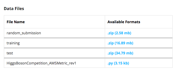
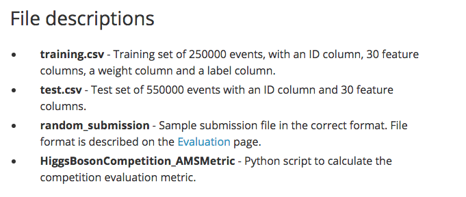
A description of the data is available from Kaggle's website for the competition . The data mainly consists of a training and a test file to make predictions and submit for evaluation. The snapshot below shows this information as it is displayed on the website. 

2 Mystery of "-999.0"

One peculiar aspect of both the training and test data is that many values are -999.0 . The data’s description states that those entries are meaningless or cannot be computed and  −999.0 is placed for those entries to indicate that .

One can analyze the nature and extent of these -999.0 entries by replacing them with "NA's" and doing this missing data analysis. We star by plotting a fraction of training data which is  -999.0 for different features and the combinations of features that occurs in the dataset

The plot to the left shows there are 11 columns where values are -999.0 with three subgroups of 1, 3 and 7 columns .  The combinations of features in the figure indicates there are 6 such combinations . Doing  same analysis on submission data gives exact same plot.  This indicates that original data can be subdivided into 6 groups, in terms of number of features having -999.0 .

Investigating the names of features with -999.0 shows that name of columns with -999.0 are  - ["DER_mass_MMC"  ],  ["PRI_jet_leading_pt"  ,   "PRI_jet_leading_eta"    "PRI_jet_leading_phi" ],   [ "DER_deltaeta_jet_jet"  ,  "DER_mass_jet_jet"  ,     "DER_prodeta_jet_jet"  , "DER_lep_eta_centrality", "PRI_jet_subleading_pt"  "PRI_jet_subleading_eta" "PRI_jet_subleading_phi" .

Diving further into technical documentation , it is evident that the group with 7 features is associated with two jets where one or no jet events are undefined . Furthermore, the group of 3 features is associated with at-least one jet production which is not defined in events when there is no jet . There are also certain observations where Higgs mass is not defined and this is not jet dependent . In conclusion, the original data can be subdivided into six groups in terms of whether or not the Higgs mass is defined and correspondingly if the event resulted in  one jet , more than one jet,  or no jet production at all.  (2 x3) . We  add two new features to incorporate this information .

3 AMS Metric

AMS is the particular evaluation metric for the competition . It's dependent on signal , background and weights associated with them in a peculiar manner as below.

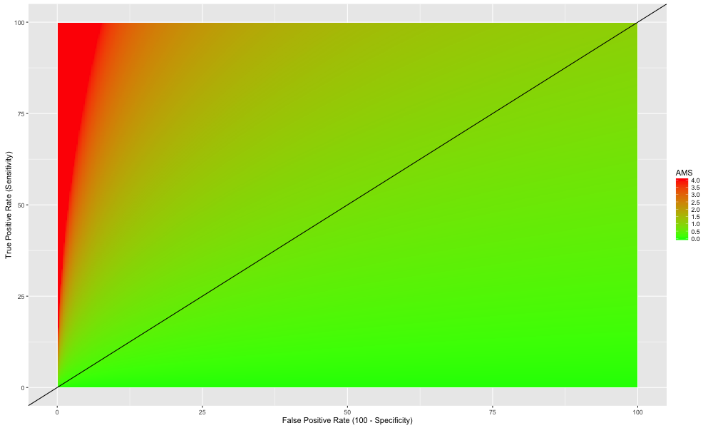
A plot of AMS for complete training data range for  s and b is shown below . AMS color is saturated for score above 4 as top leaderboard score is less than 4 and we want to concentrate on what makes those models good.

The red region corresponds to high AMS scores which are linked to low false positive and high true positive rates That is expected,  but the peculiar aspect in the figure above is that there is a range of models which can achieve top ranked score of 4 and one such model would be identifying just 25 % of Higgs signal correctly, keeping the false positive rate to 3%, and still have the same AMS score of 4.

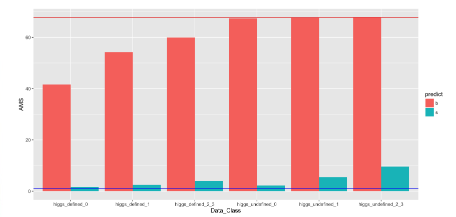
Next we investigate how much AMS score on training is influenced by performance in 6 data subgroups we identified in the last section. The red line in the previous plot is produced by a perfect prediction of the training data.The blue line below indicates AMS if every prediction is said to be a signal . For each of the data subgroups we calculate the AMS score by assigning either signal or background noise to all the events in that subgroup and using correct predictions for the rest of the data .

The figure above shows that performance on data where the Higgs is not defined has almost no effect on the AMS score if everything is classified as background signal for these subgroups.  This behavior occurs  because there is very small signal in the data where the Higgs is not defined. Moreover the weight of the signals is low and the background noise has higher weights. These three factors make  identifying everything as background noise is as good as identifying everything correctly.

Thus, classifying all events where the Higgs is not defined as background  will perform equally well in terms of the AMS score . This reduces the subgroups of data for predictive modeling to 3 that is Higgs is defined and event resulted in either one jet or more than one jet or no jet at all.

4 Data Preprocessing

We prepare our four subgroups of data each for training and test  and remove all the features which have NA's and one's which have become redundant and scale the data . Finally we are left with only 60% of original data which is useful for predictive modeling. Doing same for submission data also leaves with 60% of predictive modeling data further cementing the idea to drop NA's , keep aside Higgs mass undefined data and splitting original data into three subgroups.

5 Response

We explore response of Higgs Kaggle  which is named Label in the dataset . Plotting histogram of the weights associated with the Labels indicate Label and weights are dependent on each other . The signals exclusively have lower weights assigned to them than the background and there is no intermingling between the two Labels . This is a pretty good reason for Kaggle to not provide weights for test set !

A density plot of background signal does show some distinction between three subgroups but not obvious ones so we would leave it at that and come back if needed.

Histogram of signal shows that there are three weights or channels in which Higgs is being sought after. There are more "no jet" events with higher weights than "two or more jets" events which are larger in number but have lower weights .

6 Features

Correlation 

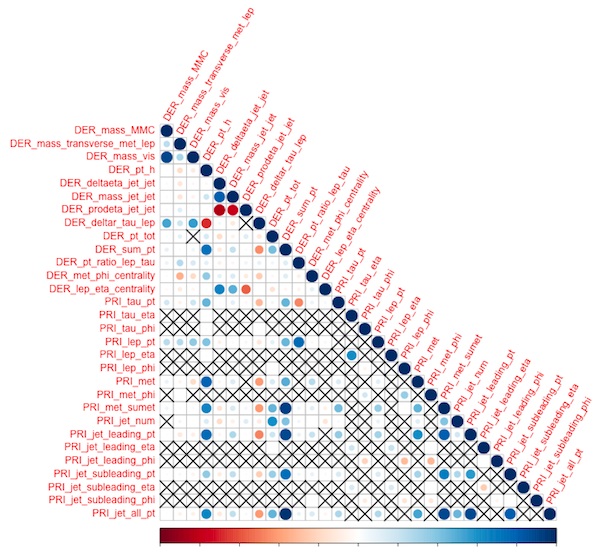
We first look at the correlation among features for the three data subgroups . The order here is {2,1,0 }. Upper triangle which corresponds to DER (derived) features in all three seems to be correlated .  These are not observations but features engineered by CERN group using particle physics. The lower right triangles which contains all PRI (primitive) features  are not correlated . It could be a good idea to drop all the engineered correlated DER features .

Principal Component Analysis  (PCA)

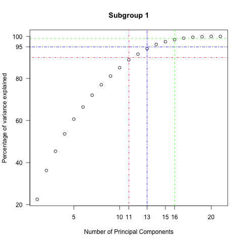
Examining the variance explained by the principal components used indicates there is a room for the reduction of features in all three subgroups . For example, for subgroup 2 , fifteen components out of 30 can explain 90 % of variance in the data and 24 components can explain 99% of variance .

 Subgroup 1  {90,95,99} % = {11 ,13,15}                             Subgroup 0   {90,95,99}% = {9 ,10,13}

PCA Eigenvectors

So our next challenge is to identify which original features do not have any influence or have very little influence in explaining the data . We start by multiplying the PCA eigenvalues and corresponding PCA eigenvectors and plotting the projections on a heat map. The product calculated in the previous step represents the transformed variance along the PCA directions . We then sorted this along the  horizontal axis  by the PCA eigenvalues' , starting  with  lowest on the left to the highest on the right . As is evident from the figure below, the lower eigenvalue transformed variance (starting from F30 and going towards F1) is zero which is what we would expect from the PCA plot from the last section

We now sort the original features along the vertical axis with respect to their contribution to the variance. We do this for the transformed variance products in descending order.  We sum up the absolute value of the contributions and not just the contribution (as a feature can have positive or negative projection indicated by red and blue colors). At the end of this process, we are left with features that contribute the least variance displayed at the bottom.

The last 9 features in the above plot stand out from the rest of features as they have white blocks or zero contribution towards first four principal components. Another important observation is that they are all  phi or eta angle features.Similarly phi and eta angles in subgroup 1 and subgroup 0 show the same behavior. In next section we will see why they are least useful in explaining the data .

Density Plots 

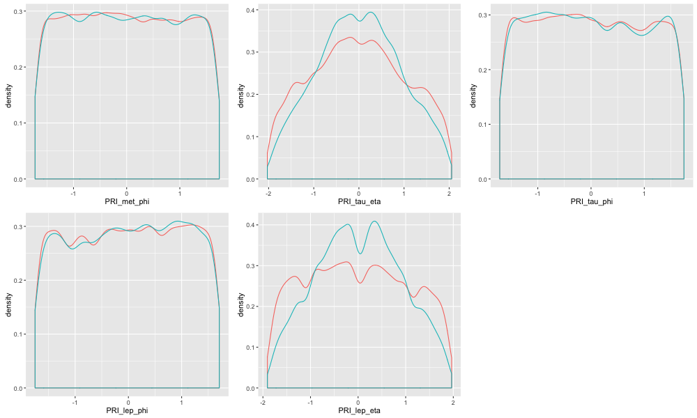
Let's look at the density plot of the last 9 whitewashed features of subgroup 2. We see they share a few common characteristics . As pointed earlier, they  are all angle features for directions of particles and jets. In the case of the 5 phi angle features they have uniform and are identically distributed over the range for both the signal and background. This is true to some extent for eta features also but for phi it is strikingly true. Conceptually it does make sense as the particles and jet would scatter off in all directions whether or not they are signals or background. Thus, the variables will follow a uniform distribution.

The plot below contrasts this uniform distribution aspect of the least influential features to the density plots of the first 9 most influential features.

The same is evident for angle features for subgroup 1 and subgroup 0.

7 Feature reduction

The last section gave us plenty to think about with respect to which features are least influential in explaining the variance. But this particular Higgs Kaggle competition's success is determined by maximizing the AMS score.  Thus discarding any features or for that sake any amount of data may not be a wise decision . But we can still use the above insights as a guide I propose the following approach.

First Iteration   

• Drop  DER features
• Drop eta features
• Drop phi  features
• Assign Background to Higgs Undefined
• Separate Predictive modeling on 3 subgroups

Second Iteration

• Drop eta features
• Drop phi  features
• Assign Background to Higgs Undefined
• Separate Predictive modeling on 3 subgroups

Third Iteration

• Drop phi  features
• Assign Background to Higgs Undefined
• Separate Predictive modeling on 3 subgroups

Fourth Iteration  (if needed)

• Assign Background to Higgs Undefined
• Separate Predictive modeling on 3 subgroups

Fifth Iteration      (if needed)

• Predictive modeling on 3 subgroups and Higgs Undefined

Sixth Iteration      (Nope. Do something else)

• Brute force on full data

8 Resultant Data for Predictive Modeling

Let’s evaluate the approach outlined above. Using only the data which matters will reduce computation power and time needed.  This model will be more accurate as it will reduce noise.  Moreover, less data to deal with means that one can try more computationally expensive models like Neural networks and SVM's and try to get lucky with automatic feature engineering .  To quantify  this benefit, we  plot the amount of data used at each modeling iteration.

9 A sample xgboost Model

We fit an xgboost decision tree model to our training data using the insights above . I chose xgboost here due to its having  low variance , low bias, high speed, and more accuracy.  We will follow the "Third Iteration" schema  from section 7 .  Let's prepare the training and testing sets by dropping the phi variables, and assigning the background noise label to data where Higgs is not defined, and splitting the data where Higgs is defined into 3 subgroups.

"AUC" is the metric of choice here as it responds well to misclassification errors.  The optimal number of trees to maximize the AUC score will be found by cross validation. We fit the whole training data to  the optimal number of trees for each dataset and make predictions for the test data to submit to Kaggle. 

The Private AMS score for this model is 3.53929 . That's satisfactory for me at the moment considering we didn't tune any hyper-parameters except for the number of trees and set the same threshold for all three subgroups. One need to do a grid search to find the three different thresholds.

We use "AUC" as our choice of metric as it responds well to misclassification errors.  We use cross validation to find numbers of trees which maximizes AUC .

We fit the whole training data to most optimal number of trees for each dataset and make predictions for test data and prepare file for submission on Kaggle.

Private AMS score for this model is 3.53929 . That's satisfactory for me at the moment considering we didn't tune any hyper-parameters except number of trees  here .  Plus we set same threshold for all three subgroups. One need to do a grid search to find the three different thresholds.

10 Conclusions

•  -999.0 are placeholders for undefined values Any attempt of imputation is plain wrong,won't work , make things bad.
• -999.0 split original data into six subgroups i.e. if Higgs mass is defined (or not) and correspondingly how many jets are formed (0 , 1 or more than 1)
• A high AMS score requires predominantly a low false postive rate and also a high true positive rate
• Setting everything to background for observations where Higgs mass is not defined has a very tiny effect on AMS score
• One can effectively do predictive modeling on three subgroups of data where Higgs mass is defined and correspondingly how many jets are formed (0 , 1 or more than 1)
• The weights and the signal are dependent on each other.
• The Higgs is being sought in three channels in the data
• The DER variables are correlated to each other and the PRI variables are uncorrelated for most part
• The angle features of phi and eta have least influence on explaining the variance
• There is only 16 % of uncorrelated data which explains most of the variance in the data
• A simple xgboost model gives a respectable AMS of 3.53929

11 Future Work

• Grid search for hyperparameters of xgboost model and thresholds
• Ensemble Methods
• Stacking
• Feature engineering
• Use "iteration 1" , "2" with the least amount of uncorrelated and significant data with more computationally expensive methods such as Neural networks and SVMs to do automatic feature engineering