Price: Machine Learning - Iowa House Price Prediction
The skills I demoed here can be learned through taking Data Science with Machine Learning bootcamp with NYC Data Science Academy.
Introduction
The aim of this machine learning project is to predict the sales prices of different homes based upon a Kaggle Dataset representing 79 explanatory variables describing every aspect of residential homes in Ames, Iowa.
The model results will be evaluated based on the Root-Mean-Squared-Error between the logarithm of the predicted values and the logarithm of the observed sales price.
Dataset
The dataset for this project was obtained from Kaggle and was divided into a "training dataset" and a "test dataset". The training data set consisted of 1460 houses (i.e., observations) in addition to 79 attributes (i.e., features, variables, or predictors) as well as the sales price of each house.
On the other hand, the testing set included 1459 houses with the corresponding 79 attributes, but without the sales price since this would be our target variable.
An analysis of the sales price provided the following:
Several data points are displayed above. Note that the average housing sale price in Iowa is $180,921.
Preprocessing
The first step in this stage of the project was to combine the "training dataset" and "test dataset" into one dataframe in order to process all the data. This would make it easier since every "process" applied to the data could be applied to both datasets at the same time.
The second step was to ascertain the number of "missing variables" in the data set. Some of the features which displayed a high number of missing variables were: "LotFrontage", "Alley", "GarageType", "GarageYrBlt" amongst many others.
The third step involved dropping all features that had more than 1000 missing variables because it was felt that this data would affect the accuracy of the model. All other features with missing values less than 1000 had those values replaced with the "mean" values of the corresponding features.
The fourth step of preprocessing involved adding dummy variables to the data steps. A large proportion of the housing features in the dataset were categorical variables. In order to better process them, I used the function "pd.get_dummies" which converts the categorical variables into a series of zeros and ones.
After all these steps were taken, the final action was to split the dataframe back into the "training set" and the "testing set".
Visualization
Several visualizations were undertaken in order to better understand the datasets.
- The target variable of the "training dataset" is the sales price of the corresponding houses. The histogram below was created to evaluate the sales price.
The housing sale price between $100K and $200K is the most plentiful.
2. Analysis of housing sales price and lot area
The chart above examines the relationship between "housing sales prices" and the corresponding "lot areas". There is no clear relationship showing above. Most of the housing "sales prices" are clustered in "lot areas" between "0" and "50,000".
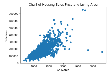
3. Analysis of housing sales price and ground living area
The sales price seems to be positively correlated to the ground living area of a house. The larger the ground living area, the larger the price.
4. Correlation heatmap
A correlation heatmap was also created using "Seaborn". This would enable one to explore what features are most important.
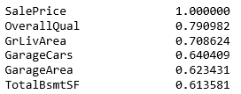
The top 5 related features most correlated to the "sale price are below:
These are:
- OverallQual: Rates the overall material and finish of the house (1 = Very Poor, 10 = Very Excellent)
- GrLivArea: Above grade (ground) living area square feet
- GarageCars: Size of garage in car capacity
- GarageArea: Size of garage in square feet
- TotalBsmtSF: Total square feet of basement area
Modelling Using the Full Feature Set
All the features were used in several different models to determine which one is the best at predicting the housing sales price. To test the models, the data was split into a "70% - 30% train test split". First the models were instantiated and then fitted. The models were fit using "X_Train" and "y_train", and then scored using "X_Test" and "y_test".
The models that were evaluated were: "Linear Regression", "Ridge", and "Lasso". The performances of the models were evaluated using the r-squared value. A high r-squared value means a higher model accuracy.
These are the r-squared related to each model:
- Linear Regression
R-squared for training dataset - 0.9467
R-squared for test dataset - 0.7996
- Ridge
R-squared for training dataset - 0.9297
R-squared for test dataset - 0.8908
- Lasso
R-squared for training dataset - 0.7835
R-squared for test dataset - 0.8205
The "Ridge" regression had the best performance with respect to to the "test dataset" with an r-squared of 0.8908.
Conclusion
In conclusion, the "Ridge" regression was the best model to predict the sales price of the "test dataset". A new dataframe with an "ID" and "SalePrice" column was created:
Greater accuracy may be derived by exploring whether any features can be removed or engineered to add more predictive value. In addition, we can determine if using a sample of the most correlated features would increase or decrease accuracy.


