Data Analysis ML: Predicting House Prices
The skills I demoed here can be learned through taking Data Science with Machine Learning bootcamp with NYC Data Science Academy.
Introduction
There has been a rise in machine learning applications in real estate. To that end, this project seeks to build a model to predict the final sale prices of each home found in the Ames Housing dataset. The data uses 79 variables to describe different aspects of the residential homes. This project will use exploratory data analysis, data cleaning, feature engineering and modeling using linear and non-linear models to achieve the goal of predicting house prices.
Modeling
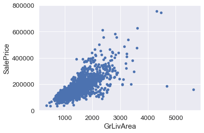
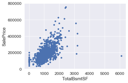
The data consists of 36 numerical and 43 categorical variables with 1460 instances of training data and 1460 of test data. The source code for this analysis and modeling can be found in Github. As a first step, the relationship between some of the numerical data types and SalePrice is explored, namely GrLivArea and TotalBsmntSF. There appears to be a strong linear relationship between GrLivArea and SalePrice. There is also a somewhat linear relationship between TotalBsmntSF and SalePrice, however, in certain cases, SalePrice seems to have less of an impact than TotalBsmntSF.
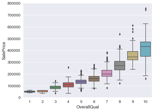
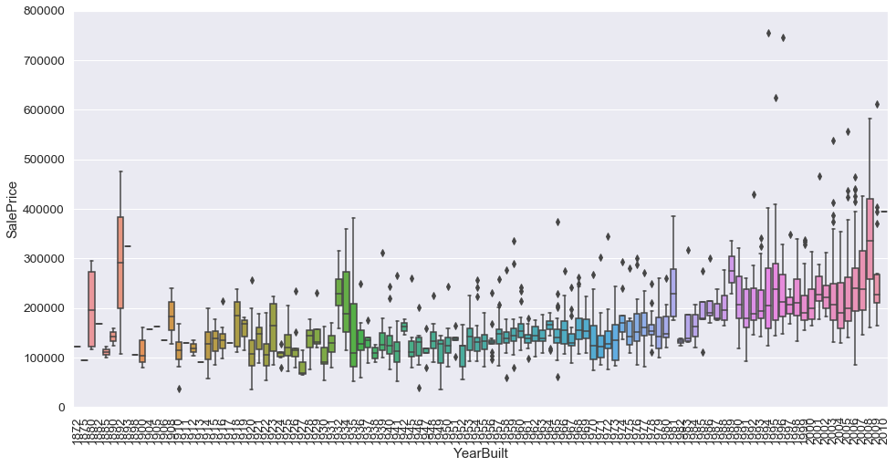
In addition to analyzing and exploring numerical variables, categorical variables are also explored namely, OverallQual and YearBuilt. The boxplot below demonstrates that the OverallQual is directly representative of a SalePrice. Better the quality, higher the SalePrice. OverallQual and YearBuilt also seem to be related to SalePrice. The relationship seems to be stronger in the case of OverallQual, where the box plot shows how sales prices increase with the overall quality.
In order to understand how the dependent variable and independent variables are related, a correlation matrix heatmap is prepared to visualize the correlation between features. The correlation heatmap below shows how strongly pairs of features are related. To further narrow the dependency and zoom into the 10 most correlated features, a correlation matrix heatmap of top 10 correlated features is shown.
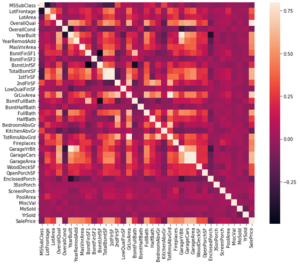
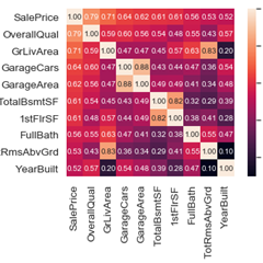
- 'OverallQual', 'GrLivArea' and 'TotalBsmtSF' are strongly correlated with 'SalePrice'.
- 'GarageCars' and 'GarageArea' are also some of the most strongly correlated variables. However, the number of cars that fit into the garage is a consequence of the garage area.
- 'TotalBsmtSF' and '1stFloor' also seem to strongly correlated and can be merged as one feature.
- 'TotRmsAbvGrd' and 'GrLivArea', are also correlated and can be merged as one feature
- 'YearBuilt' is slightly correlated with 'SalePrice'.
With the data exploration completed, the next step is to clean data and impute missing values. The table below shows the missingness statistics of the features in the dataset. Most of the missing entries are due to the house missing a feature: for example, garage, basement, pool, fence, alley. These can be replaced with binary values. Other variables such as LotFrontage, MasVnr, are imputed using the neighboring median value.
| Total | Percent | |
|---|---|---|
| PoolQC | 1453 | 0.995205 |
| MiscFeature | 1406 | 0.963014 |
| Alley | 1369 | 0.937671 |
| Fence | 1179 | 0.807534 |
| FireplaceQu | 690 | 0.472603 |
| LotFrontage | 259 | 0.177397 |
| GarageCond | 81 | 0.055479 |
| GarageType | 81 | 0.055479 |
| GarageYrBlt | 81 | 0.055479 |
| GarageFinish | 81 | 0.055479 |
| GarageQual | 81 | 0.055479 |
| BsmtExposure | 38 | 0.026027 |
| BsmtFinType2 | 38 | 0.026027 |
| BsmtFinType1 | 37 | 0.025342 |
| BsmtCond | 37 | 0.025342 |
| BsmtQual | 37 | 0.025342 |
| MasVnrArea | 8 | 0.005479 |
| MasVnrType | 8 | 0.005479 |
| Electrical | 1 | 0.000685 |
| Utilities | 0 | 0.000000 |
With the data cleaned and missing data imputed, there can be introduced some feature engineering to better set up the data for modeling. Some features such as Street and Utilities can be dropped since they are not correlated to SalePrice. Other features such as floor space, bathroom, and garage features can be combined to form a single feature. Some features such as KitchenAbvGr and HalfBath can be converted to categorical features so they can be easily recognized by the model. Finally, dummification of the categorical variables is done to be able to use, linear regression models.
The data is now ready for modeling. Both linear and non-linear models are used to predict SalePrice. The training data is divided into a 80-20 split. The linear models used are Ridge, Lasso and ElasticNet regression and the non-linear models used are Support Vector Machine, Random Forest and Gradient Boosting. The table below shows the R-squared and Mean Square Error values for the different models.
gradient boost    0.102793
ridge             0.117614
lasso             0.119479
ElasticNet        0.119755
forest            0.138547
svm               0.764708
dtype: float64
svm               0.001828
forest            0.001879
gradient boost    0.002742
ridge             0.011920
lasso             0.013152
ElasticNet        0.013267
The following table shows a snippet of the predicted house SalePrice given by different models.
| Id | ridge | lasso | ElasticNet | forest | svm | gradient boosting | |
|---|---|---|---|---|---|---|---|
| 0 | 1461 | 118514.7 | 120398.9 | 120314.9 | 77527.7 | 122264.0 | 128603.0 |
| 1 | 1462 | 157988.8 | 141466.7 | 141251.2 | 194734.2 | 153565.8 | 165000.2 |
| 2 | 1463 | 174265.2 | 175816.3 | 175705.7 | 163086.4 | 178705.7 | 188985.5 |
| 3 | 1464 | 196641.3 | 198890.0 | 198776.9 | 200336.2 | 185670.5 | 202622.6 |
| 4 | 1465 | 198854.4 | 193911.5 | 193816.0 | 151076.3 | 192523.4 | 189557.4 |
| 5 | 1466 | 170228.8 | 170645.4 | 170670.6 | 186008.3 | 183257.2 | 182585.4 |
| 6 | 1467 | 180233.2 | 188000.3 | 188074.7 | 248834.1 | 177754.4 | 178314.7 |
| 7 | 1468 | 163638.1 | 164375.1 | 164404.1 | 163461.6 | 174988.8 | 169385.4 |
| 8 | 1469 | 188252.2 | 196122.7 | 196156.1 | 175741.5 | 184451.5 | 176197.4 |
| 9 | 1470 | 120014.7 | 117923.8 | 117890.8 | 118968.2 | 124419.1 | 125261.3 |
Conclusion
Linear models such as Ridge, Lasso, ElasticNet are simple to implement and easy to tune and performed relatively similar. Non-linear model, SVM, reported the least mean square error and the highest R-squared score.

