Using Data to Predict House Prices in Ames, Iowa
The skills the authors demonstrated here can be learned through taking Data Science with Machine Learning bootcamp with NYC Data Science Academy.
Overview
Our team worked on a Kaggle competition to use Machine Learning techniques to predict house prices in Ames, Iowa. While the data was fairly linear and our multiple linear regression models performed quite strongly, our team additionally explored tree-based models and gradient boosting to further fine tune our predictions. After our project deadline, our best-performing model, a Ridge-regression, earned a Kaggle score - Root Mean Squared Logarithmic Error (RMSLE) of 0.12509, which placed us in the top 13% of submissions.
Data Science Background
As we set out to determine which features of the house were the most important determinants of house prices, we first needed to familiarize ourselves and clean the 79 features provided. The features were a mixture of numerical data including the lot’s area, basement’s square feet, and the number of kitchens, in addition to categorical variables like the neighborhood, the type of sale, and even the roof’s material.
Early analysis explored the data’s missingness, redundancy, and skewness, among other facets, to best clean and engineer new features. With multiple cycles of analysis and engineering throughout the process, we implemented linear regression and classification models to find solutions to high dimensionality, outliers, and multicollinearity.
Data Exploration
Because the data provided so many features, we aimed our beginning-stage exploration at identifying predictive power. We looked specifically at low variance, redundancy, and missingness in individual features.
Using Data to Analyze Variance
When analyzing low variance, we found that multiple columns, for example ‘Alley’ (whether a home has an alley or not adjacent to the property), could be seen as a binary “Yes” or “No”. The column ‘Alley’ contained all “Yes” answers except for 91, only 6% of the data. Worse, only 32 rows in ‘Heating’ held an answer other than “GasA”.
Even still, only 7 homes recorded a “Yes” in the ‘Pool’ feature (whether a home has a pool or not), meaning 99.5% of the homes in our data do not have a pool. To include this particular pool column could potentially lead to an overfit model, since the feature is so heavily skewed to one side, “No”. While we could propose dropping such columns with extremely low variance, we could also move to use a penalized model like Ridge or Lasso to whittle down our excess of features.

Using Data to Analyze Redundancy
Next, our team took a look at features that might be redundant, those that could possibly be easily explained by another feature. First we compared ‘External Quality’, rated on a scale from “Poor” to “Exceptional”, against the year the house was built, ‘Year’. As expected, the concentrated areas of each rating increase along the year scale as the rating increases. This would make sense as the older a home is, the more likely the exterior is to be weathered and aged from the elements.
A similar trend was discovered when analyzing ‘Foundation’ types across the decades. Before the 1940s, brick was often the foundation of choice; however between 1940 and 1990, cinder block swiftly became the material of choice. Then another swift shift in materials seems to occur around 1990, with nearly all homes having a foundation made out of poured concrete.

Right: Foundation type against year built and the sale price.
The danger of redundancy is the loss of independence, one of the assumptions of linear regression. This could lead to highly inflated and misleading coefficients from an MLR model. Our team discussed options including throwing out possibly redundant features or instead choosing a penalized model to specifically target inflated coefficients from multicollinearity.
Using Data to Analyze Missingness
Missingness occurs when at least some of an observation’s values are not present within the dataset. We set out to identify which columns contained missing values, and understand the patterns of missingness within those columns.

High Proportion of Missingness:
For the features 'PoolQC', 'MiscFeature', 'Alley', and 'Fence', there was a high proportion of missingness in these columns, with “NA”s comprising of up to 99.5%, 96.3%, 93.7% and 80.7% of the column values respectively.
Values Missing at Random:
Values missing at random are when the data is dependent on variables for which we have complete information within our dataset. We identified that missingness within 'FireplaceQu' (Fireplace Quality) corresponded to houses in which the 'Fireplaces' feature was “0” (i.e. the house does not have a fireplace). 'LotFrontage' appeared correlated to 'LotConfig', while 'GarageCond', 'GarageFinish', 'GarageQual', 'GarageYrBlt' corresponded to value “NA - No Garage” in 'GarageType'.
Values Missing Completely at Random:
Values missing completely at random are values in which the piece of data is neither related to observed variables nor related to the unobserved variables of interest. The missingness within features in relation to Basement ('Bsmt') and 'Electrical' did not seem to have any clear correlations to other columns within the dataset.
Data Cleaning and Feature Engineering
Now taking into account the information and patterns when visualizing and investigating the data, we conducted data cleaning and feature engineering to ready the data to feed into machine learning models for price prediction.
We expected a linear relationship in regards to the features of the houses in relation to the sale price (i.e. the larger the area of the house, or the higher the overall quality, the higher the sales price of the house).
Using Data to Analyze Outliers
In order to find the best fit line that is representative of the data, we also wanted to look at outliers which do not align with the values in the dataset.
For example, we expect that as the living area of the houses increase, the sale price of the house will increase as well. However we identified two observations with large living area but unexpectedly low sale price. Oddly, these two observations also had a high overall quality rating, but did not correspond with a higher sale price.
We decided to remove these two observations from the modeling set.

Using Data to Analyze Feature Manipulation
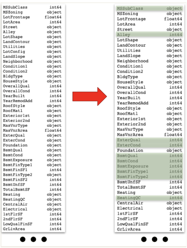
Depending on the model selection, manipulating the data types of certain features improved accuracy. For other models, the change was redundant and not necessarily needed. For example, ‘MSSubClass’, a numerical category for dwelling type, held an int64 data type, yet the relation between code 20 homes, 1-story 1946 and newer homes inclusive of all styles, versus code 40 homes, 1-story with finished attic and all ages included, up to a score of 190 isn’t necessarily a linear relationship that the numerical data type might force. For our linear regression models, we experimented with manipulating ‘MSSubClass’ to a categorical type and dummifying the feature. This was not necessary, however, for our tree based models as it naturally treats each unique value as a category.
Other features received the opposite treatment, shifting from an object to an integer. The features ‘ExterQual’, ‘ExterCond’, ‘BsmtQual’, and others measured traits like quality on a ranked scale, from “Poor” to “Excellent”. To provide a linear relationship to these ratings, informing the model that “Fair” is closer to “Poor” than “Excellent”, we manipulated these features into an integer type.


Using Data to Analyze Imputation
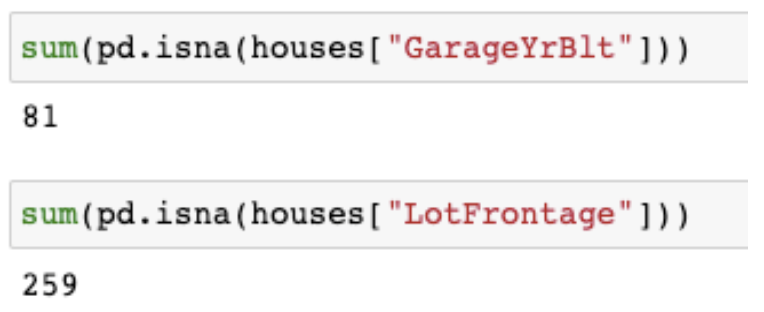
Missingness in features like 'GarageYrBlt' (the year the garage was built) and the total 'Lot Frontage' (linear feet of street connected to property) required different treatments.
For the mentioned garage feature, if the home did not have a garage, there would be no year recorded for one to be built. We imputed a value of 0 to distinguish these homes as not having garages since the feature was an integer datatype. This imputation was less necessary for our tree models.
Missingness in the 'Lot Frontage' feature, however, appeared to be instances of absent data. To salvage these 259 lines, we grouped by 'Neighborhood' then binned a similar feature, 'LotConfig' (the configuration of the lot, e.g. a corner lot or inside lot), and imputed the respective average frontage to each missing entry.
Using Data to Analyze Models
Ordinary Least Squares

After taking the log of the target sale price, we fit a multiple linear regression model to our data. Because we had all features included, multicollinearity and an overfit model were expected. By taking the score of our train set and test set, we see this low complexity model resulting in a very wide difference between scores.
Additionally, comparing the R squared scores of a feature against the rest, quite a few scores reach the top or come very close to a full score. This was yet another clue that certain features could be explained by others and that a penalization to our linear model was needed to reduce inflated coefficients.

Lasso Regression
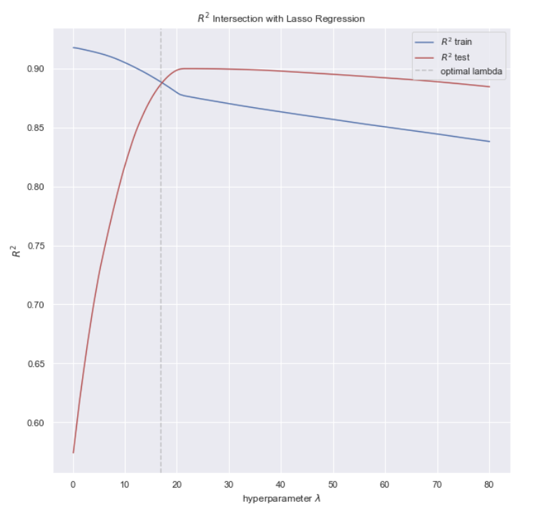
Because there were so many features, our team additionally tested a Lasso model to guide feature trimming. The graph below shows the significant drop of many features’ coefficients, a sign their slope was greatly inflated from multicollinearity.


To find the best lambda, we found the cross where the model no longer overfits (the left side of the gray dashed line, where train scores perform well yet test scores do not) and before the model begins underfitting (the right side of the gray line, where test scores now outperform train scores). Here where the train and test scores converged we extracted our lambda. As the lambda parameter increases, the model slowly worsens in accuracy as the penalty defaults to the null model and removes any affect the coefficients added.
Random Forest

While previously for our linear models we had taken the log of our Sale Price target, for tuning our Random Forest model we found the log transformation actually weakened the model. This may be that Random Forest is a nonlinear model and can handle far better a nonlinear relationship to the target.
Additionally, when we analyze the rankings of feature importance (see figure to the left), 'OverallQual' greatly surpasses every other predictor.
Gradient Boosting
Hyperparameter tuning quickly grew to a task fit better for grid search than manual manipulation. Previously Lasso and Ridge required a lambda parameter, the penalty; but for our Gradient Boosting model, parameters including number of trees, learning rate, maximum depth, and maximum features all needed testing.
Below is a sample grid search performed for our gradient boosting model. With more time, our team would have hoped to tune and feature engineer further to strengthen the gradient boosting model.

Final Results

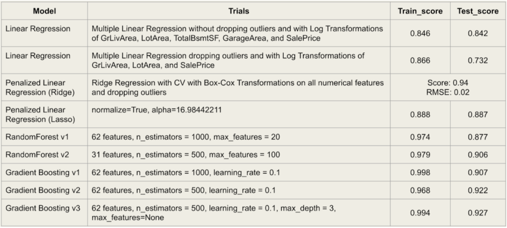
While our tree-based models did not receive as much time with hyperparameter tuning and data manipulation as our linear models, they still quickly improved with only minimal tuning. Yet, our best scoring model remained one of our Ridge models. With more time we would have liked to explore stacked models and further strengthen our models to outliers.
For housing prices, human subjectivity ('OverallQual') was frequently the largest determinant. Following shortly behind overall quality were often features measuring square footage, but quite a few other subjective categories also made it to the top depending on the model. 'ExterQual' judged on a scale of 1-5 from “Poor” to “Excellent” the quality of the material on the exterior. This feature rising to the top of feature importance rankings implies home buyers are fairly swayed by outward appearances as well.


