Predicting House Prices with Machine Learning Methods
The skills I demoed here can be learned through taking Data Science with Machine Learning bootcamp with NYC Data Science Academy.
LinkedIn | GitHub | Email | Data | Web App
Background
The goal of this project was to compete in an introductory Kaggle competition to predict the price of houses using the Ames Housing data set. This data set consists of just about every feature you can think of to describe homes sold in Ames, Iowa. It has a total of 79 predictive variables with a mix of categorical and numerical features. Many features are highly related, with 9 variables alone describing different aspects of the basement.
The competition evaluates submissions based on RMSLE (Root Mean Squared Log Error), which uses the log of predicted and actual target values so that errors in predicting cheap or expensive houses will impact the score equally. Building good predictive models requires advanced machine learning regression algorithms and gathering an excellent understanding of how features relate to sales price and impact the models.
Iterative Process
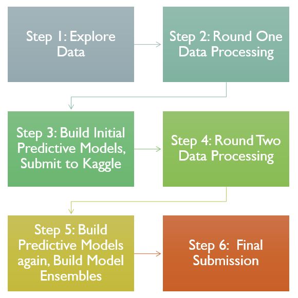
This project generally followed the below order of exploring the data to gain an understanding of how it looks, conduct some initial data processing based on intuition on how I can improve the models, build initial models and score them. After seeing how the models perform, I went back around to the data processing step to see how I could improve it and then rebuilt models and see how they improved. Finally I made ensembles of the final models using two different methods (averaging and stacking) and submitted the final scores for evaluation.
Data Exploration
Goals:
- Look at relationships between features and the target variable
- Find variables with a strong correlation with the target variable
- Explore multi-collinearity between predictor variables
- Opportunities for feature engineering or feature selection
- Explore the shape of the data
The data exploration stage is an opportunity to get an idea of the relationships between features and the target variable, to find strong correlations with the target variable. Additionally evaluating possible feature engineering options or features that can be dropped is also beneficial. This stage also yields information for the data processing stage about how the data needs to be processed before building models.
Above is a correlation matrix of the top 5 positively correlated features. From it, we can see that multi-collinearity is already evident in this subset of the features. In general, many of the predictors in the data set exhibit some relationship. The features that refer to different aspects of the same house amenities have strong relationships.
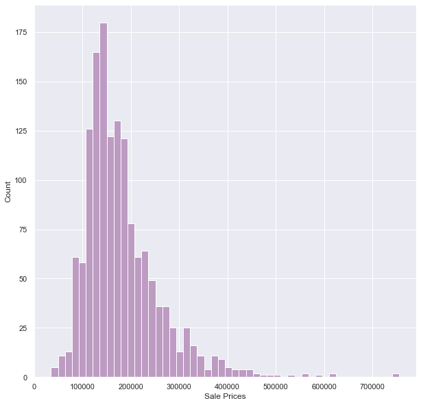
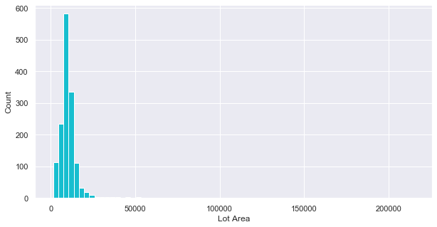
A handful of variables had a significant skew to the right, with a long tail for higher values, as can be seen in the above histogram of sale prices and the below histogram of Lot Area. In the final models, the log of variables like these were used so that high values would hopefully cause less of a bias in the models
Categorical variables were tougher to explore in mass, but made up about half the data set. The above graphs show two categorical features with the strongest relationship with sale price (as determined by later feature importance exploration in the intermediary models).
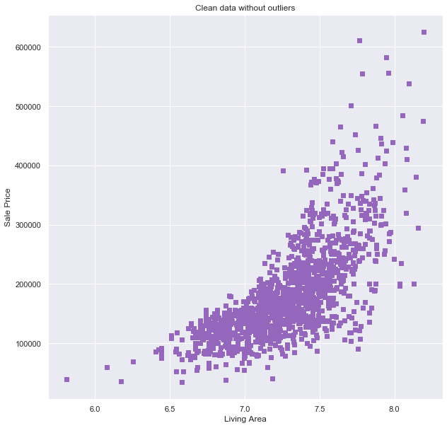
Outliers are another source of potential bias in the final models. While processing my data I decided to remove very large houses (‘Ground Living Area’ > 4,000) or houses that sold for very high prices (‘SalesPrice’ > 700,000) to reduce bias. This only removed 4 observations from the data set.
Data Processing
This phase of the project involved the following major steps:
- Categorical Variables: Dummify / Encode
- Handle missingness
- Feature engineering
Once the models were built and evaluated, I went back to the data processing stage. The following steps were decided to be beneficial to improving the model:
- Feature Selection for important variables
- Removing outliers
- Transform skewed variables
Models
The models built to predict housing price included MLR, Penalized Regression, Random Forest, Gradient Boosting, and XGBoost. Overall, XGBoost performed the best, even compared to ensemble models (just barely). Below I compare the results from the different models.
Linear Regression Models
- Checking the assumptions of MLR confirmed the data did fit a linear regression task
- Required dummification: 79 variable turns into 250+
- Penalization reduced the effects of multi-collinearity on the model
- Best performance from ridge regression
Tree Based Models
- No dummification required
- Feature Importance
- Built custom scoring method to use RMSLE as the gridsearch/cv tuning metric
- Marginal improvement in CV results, but vastly improved how robust the models were when submitting on Kaggle
Submission Results
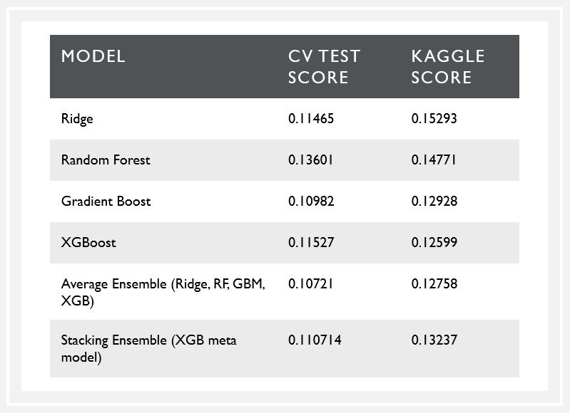
The Average Ensemble model had the best performance on my test set, but it was narrowly outperformed by the XGBoost model on the Kaggle leaderboard. Averaging can help reduce overfitting of any one model. Stacking Ensemble in theory builds on the different strengths of different models. Its poorer performance suggests to me that the base models may use similar information to predict values.
The best Kaggle score for the XGBoost model scored in the top 25% percent on Kaggle (placed #1225).
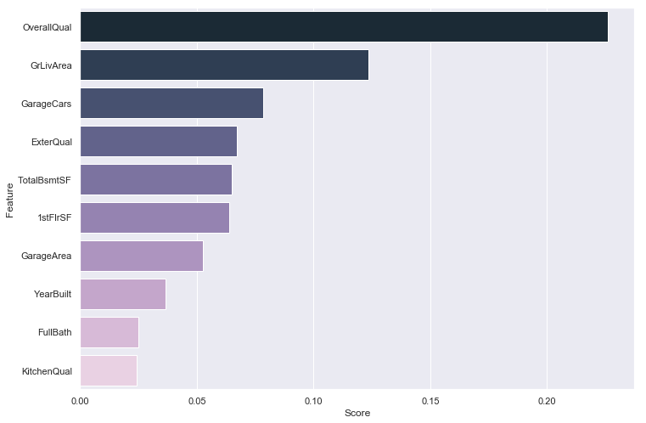
The below graph shows the feature importances in the XGBoost model. The ‘Overall Quality’ feature was the single most important predictor in every model. Other important variables include other quality-related features and size-related features.Interestingly, most of these variables also showed up with the highest correlation with sale price in the initial data exploration.
Conclusion
- There were diminishing returns on subsequent models, especially on tuning a single model for better performance
- All models performed better on the unseen/set aside test set than on predicting the Kaggle test data set
- Improvements may include more experimenting with how changes in data processing influences model performance.
- Additionally, there were more types of models or variations for model ensembling I was interested in applying to this data set that realistic constraints didn’t allow for.


