Solar-California Renewables: predicting solar generation
The skills I demoed here can be learned through taking Data Science with Machine Learning bootcamp with NYC Data Science Academy.
California is leading America and the world on clean energy
Over the past 10 years, California has established itself as a prominent leader in adopting and implementing ambitious clean energy especially solar energy policies. California matters – economically and environmentally – not only in the American but in the global context. If California were a country, it would be the world’s 5th largest economy, bigger than the UK, France, or India.
The recent Renewables Portfolio Standard implemented in 2018 requires that 50% of California's electricity come from zero-carbon sources by 2025, 60% by 2025, and 100% by 2045. The cumulative result of these bold policies and unprecedented private investment is encouraging. Over the last decade, California was able to steadily reduce the physical volumes of fossil fuel-derived generation by about 25% while growing the economy by 40%.

California's transition towards renewable energy comes with significant challenges on the economic, technological, and regulatory fronts. My Shiny app investigates some of these challenges and explores a machine learning approach to address one of the biggest uncertainties: the variability of solar generation.
The project has two specific objectives:
- To identify the most accurate forecasting method and to assess possible economic benefits,
- To provide a primer on using various techniques for autoregressive time series forecasting.
Current challenges: too much solar?
About 80% of California’s energy is delivered by the California Independent System Operator (CAISO), a non-profit organization responsible for balancing electricity supply and demand and ensuring California’s grid reliability. The source data for the Shiny app came from the 10 years of hourly electric generation published by CAISO (a sample of the daily data).
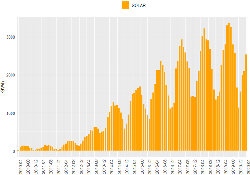
While the annual trend looks like a steady buildup of the renewable generation, monthly breakdown shows significant seasonal variation. Solar generation spikes at summer to about 3 TWh/month with close to 14 hours of daylight (and higher intensity) and goes down to about 1 TWh/month in December. Fortunately, seasonal solar production is peaking in sync with surging summer demand driven by air conditioning:

Yet despite this resounding success at the big picture level, policymakers, media, and CAISO itself describe the situation as alarming. You can stumble upon recounts of how California grapples with ever-growing amounts of renewable energy, and what to do with the solar energy that CAISO has to curtail.
The Duck Curve for Solar Generation
The problem becomes apparent when we zoom in to the hourly level. Solar generation in California peaks at 2-4 pm, while traditional power plants are turned down to the minimum. From around 4 pm to 8 pm, solar generation declines to zero – exactly at the time when demand is peaking, which requires large and fast power ramping from traditional sources.
This is what April 30, 2020 looked like at CAISO:

Note also that the short-term power storage capacity (so far confined largely to lithium ion technology) is too small to smooth out this daily solar cycle in a meaningful way. In other words, today, energy needs to be consumed the instant it is generated.
CAISO coined the term ‘the duck curve’ to describe the formidable intraday swings in the net load (total demand less solar and wind generation).
This is how the net load on the same day (April 30) has changed from 2010 to 2020:

Over the past decade, the duck’s belly has got deeper and deeper, and today these swings amount to 15GW capacity and more in a matter of 3-4 hours. To put this into perspective, this is roughly equivalent to the total installed capacity of a medium-sized country such as Switzerland or Israel. In other words, CAISO has to turn an entire country’s electric generation on and back off, every day, to smooth out the solar output. This is the greatest challenge facing renewable energy in California today.
Forecasting Solar Generation
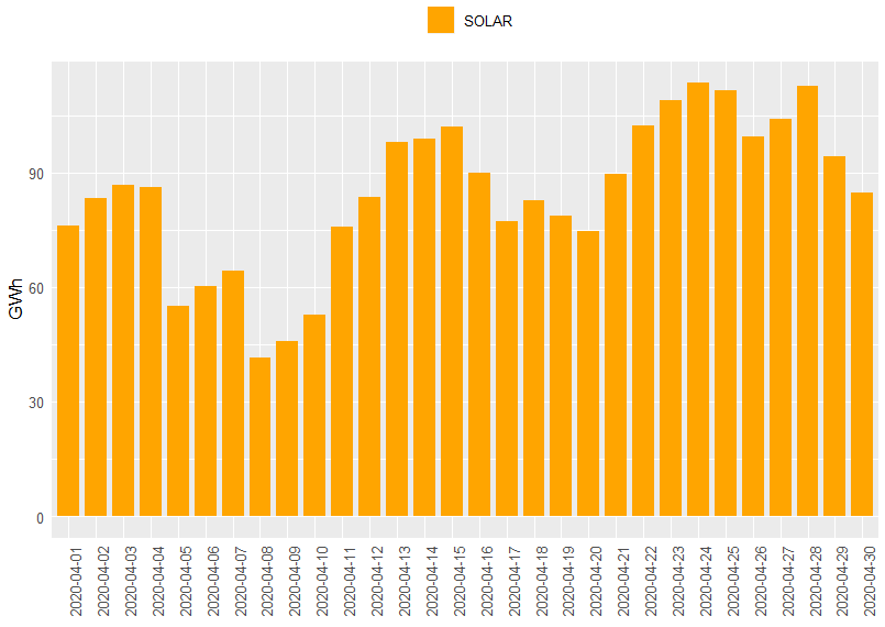
And yet there is another aspect of solar that makes it even more complicated for CAISO: the poor predictability. Not only is solar generation intermittent, it is also inherently irregular, affected by the cloud cover and numerous other factors such as dust, precipitation, and temperature. Within a typical month, the actual daily solar generation may fluctuate by 30-50%:

CAISO needs to forecast this volatile supply to balance the entire system and ensure grid stability. That’s why predicting solar and wind generation is at the center of CAISO’s attention. CAISO runs many different types of forecasts ranging from 15 minutes ahead to 1 hour ahead to 24 hours and beyond.
The goal of this project is to identify the best method of predicting the solar generation for the purely autoregressive model in the absence of any external inputs. Of the 5 forecasting methods analyzed, the best accuracy was achieved by an ensemble of a classical autoregressive SARIMA and a recurrent neural network.
On average, this ensemble improved forecasting accuracy by about 25% (0.07 GW) compared to the best non-machine learning method (Differencing):

For CAISO, this improved accuracy would translate into less reserve capacity requirements. California’s current Capacity Procurement Mechanism sets the price for extra capacity at $75 kW-years, which would translate into at least $5 million annual saving for CAISO.
Conclusions
Solar generation is the centerpiece of California’s bold clean energy policies. However, it is intermittent and irregular. My Shiny app shows that uncertainty in solar generation forecasts can be reduced significantly by machine learning methods, which would lead to sizable economic benefits for CAISO.
Autoregressive time series forecasting: A technical primer
The dataset for this project consists of 87,936 timesteps: slightly over 10 years of hourly electricity generation data for the period of April 20, 2010–April 30, 2020 provided by CAISO.
Each forecasting model was trained on data ending on December 31, 2018. Incremental retraining was not implemented – both autoregressive SARIMA and RNNs took from 10 to 20 minutes to train on Tesla P100 GPU, so retraining for each new timestep was not feasible.
All forecasts are built on actual hourly series for the 1-hour ahead horizon. Models’ performance is tested and compared on 2019-2020 test data, i.e. completely out-of-sample.
Naïve Forecast of Solar Generation
In time series forecasting, the naive prediction of F(t+1)=F(t) often serves as a basic benchmark because it turns out surprisingly hard to beat (especially in aperiodic, low signal-to-noise environments). CAISO uses such benchmarks (also called persistence forecasts) extensively in tactical planning.
Below is a naïve forecast of the solar generation for the last 3 days of April 2020, a typical picture of how volatile the generation is. The MAE of the naïve forecast over these three days is 0.87 GW.

Differenced Forecast
A slightly less naïve approach, applicable only for periodic series, relies on smoothing the signal as compared to previous periods:

This forecast does not learn any patterns directly from the data. This is essentially a potentially moving average MA(1) process for the once-differenced I(1) series with fixed coefficients. A grid search of relevant parameters produced the optimal configuration, which turned out to be very simple:

This is essentially forecasting the next hour as the current generation (naïve) adjusted for the difference in generation between the same adjacent timesteps 24 hours ago. We can see from the graph that this 24-hour differencing forecast fits the data remarkably well, producing a simple and reliable benchmark.
The three-day MAE is 0.33 GW, which is less than 40% of the naïve error.

SARIMA Solar Forecast
My third approach was to implement a classical SARIMA autoregressive model, which was motivated by the following:
- The strict 24-hour period warrants at least one order of differencing.
-
When there is inertia and mean-reversion in the underlying data-generating process, it is best described by a moving average MA(q) process. There is clearly inertia in cloud cover, precipitation, and temperature, which tend to affect solar generation in multi-hour stretches.
- The regular autoregressive part of the process is inferred from the shape of ACF/PACF correlograms and tested by a grid search.
The raw hourly generation is of course highly autocorrelated:

The raw process is highly non-stationary, with trend and seasonality. We achieve quasi-stationarity only after double differencing by 24 and 1 periods. The ACF for this I(2) series shows strong autocorrelation for h=1 and h=24 time shifts:

We can conclude that the differenced series is probably a MA(1) process. This means that the model will adjust its predictions by some portion of the error it made in the previous time step, which may have been caused by a random shock such as cloud cover.
Grid search for the best configuration produces the following compact SARIMA:

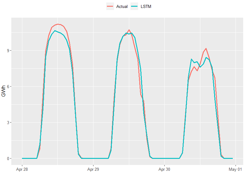
SARIMA model works particularly well in this case because solar generation is inherently periodic and strongly autocorrelated. This is our best forecast with MAE = 0.25 GW (all metrics are out-of-sample):

Recurrent Neural Network
Finally, I deployed an RNN-based neural network that was trained on approximately 2.5 years of data, from June 2016 to December 2018, and tested on 2019-2020 data. Each training sample consisted of 48 hours of historical generation and the network was trained to predict the following hour’s generation.
RNN's error was worse than SARIMA's, at 0.33 GWh for our 3-day sample. Apparently, there is little non-linearity nor long-term dependencies, which RNNs are very good at.
In particular, RNN seems to miss the peaks of the cycle more than SARIMA. If this bias proves to be systematic, it may be possible to compensate for.

Ensemble
The best accuracy is obtained by averaging the SARIMA and RNN models. A simple 50/50 average achieves a sizable decrease in Mean Absolute Error compared to either SARIMA or RNN alone.
Note that all of the models above are autoregressive. Including exogenous predictors such as weather forecasts would further improve the accuracy. However, it would imply additional operational complexity for CAISO since the cloud cover, precipitation and temperature forecasts need to be accounted for each of the 700+ of California’s solar sites.
To learn more about how to build a SARIMA model with statsmodels API, how to deploy a time-series data pipeline in TensorFlow, or how to set up a learning rate decay schedule, please visit the project’s github.

