US Smoking Rates, Cancer and Cigarette Tax

Contributed by Brain. Brain took NYC Data Science Academy 12 week full time Data Science Bootcamp program between Sept 23 to Dec 18, 2015. The post was based on his first class project(due at 2nd week of the program).

Overview

This project utilizes publicly available data to visualize temporal trends of smoking rates, lung/bronchus cancer incidence and cigarette tax across 6 geographic regions within the US.  Smoking is associated with negative health outcomes such as lung cancer and excise tax on cigarettes is a public health approach to lower smoking rates within the US.^{1 ,2}  Immediately below, you will view a series of questions with each followed by several data visualizations.  Details on data and methodology are located at the end of this blog post.  All data loading, manipulation and visualization is performed using the R statistical software and the code is located at the end of this blog.

Cigarette Tax = Smoking Rates?

Figure 1: Cigarette Tax ($ Per Pack) Over Time    

Figure 1 shows that cigarette taxes increase over the time period 1999 - 2012 across all regions within the US.  You will notice that the pacific and northeast regions have the highest state level excise tax on cigarettes whereas the NC-KY-GA  and south regions have the lowest amount of state level excise tax across this time period.

Figure 2: US Region Current Smoking % Over Time

Figure 2 shows that smoking rates across all regions within the US decrease over the 199 - 2010 time period.  The NC-KY-GA and south regions have the highest current smoking rates whereas the northeast and west have the lowest current smoking rates across this time period.

Figure 3: Current Smoking (%) & Cigarette Tax in the US

Figure 3 incorporates 3 dimensions in order to visualize the relationship among current smoking percentage and cigarette tax across time.  You will notice that regions (such as the northeast, west and pacific)  with higher cigarette taxes tend to have lower current smoking percentages across time compared to regions with lower cigarette taxes such as NC-KY-GA and the south.

Smoking Rates = Lung/Bronchus cancer rates?

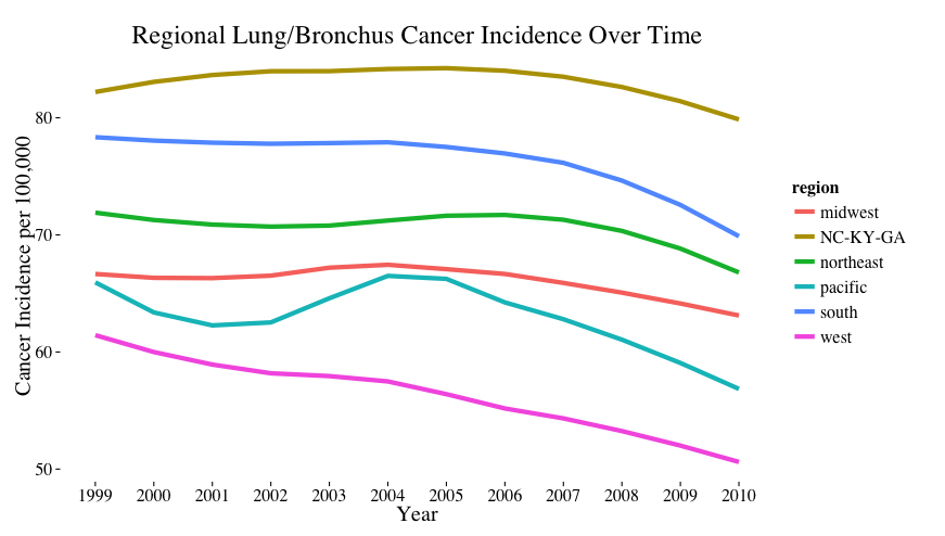
Figure 4: Regional Lung/Bronchus Cancer Incidence Over Time

Figure 4 identifies lung and bronchus cancer incidence for each of the 6 US regions across the 1999  - 2010 time period.  You will notice that the NC-KY-GA and south regions have higher lung/bronchus cancer incidence rates compared to the west, pacific and northeast regions.

Figure 5: Current Smoker % and Cancer Incidence Over Time

Figure 5 incorporates the relationship between current smoking percentage and lung/bronchus cancer incidence for each of the six regions across the 1999 - 2010 time period.  You will notice that regions with higher current smoker percentages such as the NC-KY-GA and south regions have higher lung/bronchus cancer incidence compared to regions with lower current smokier percentages such as the west and pacific.  The northeast seems to contradict this trend by having low current smoker percentages but with a moderate lung/bronchus cancer incidence rate.

Which regions have the highest per capita average health expenditures attributable to smoking?

Figure 6: Health Expenditure Attributable to Smoking 

Figure 6 identifies the per capita health expenditures attributable to smoking for each of the 6 regions.  You will notice that the northeast has the highest per capita health expenditures attributable to smoking whereas the NC-KY-GA region has the lowest per capita health expenditures attributable to smoking.

Data & Methodology

• Data Source: Center for Disease Control and Prevention
  • Behavioral Risk Factor Surveillance System
  • State Tobacco Activities Tracking and Evaluation System
  • Smoking-Attributable Mortality, Morbidity, and Economic Costs
  • enigma.io/publicdata/
• Metrics
  • Smoking Rates– “Current Smokers”
  • Cancer – “Lung and Bronchus Cancer Incidence”
  • Smoking Attributable Economic Costs – “Excess health care expenditures attributable to smoking”
    • Ambulatory, Hospital, Nursing, Other, Prescription Drugs
• Population
  • All genders, All ages, All races, All education

• Geographically Categorized Analysis Groups:
  • Northeast: PA, NY, NJ, CT, MA, RI, VT, NH, ME
  • Midwest:ND, SD, NE, KS, MN, IA, IO, MO, WI, IL, IN, OH, MI
  • South: TX, OK, AR, LA, MS, AL, GA, FL, SC, NC, TN, KY, WV, VA, DC, MD, DE
  • Pacific: HI, AK
  • West: MT, WY, CO, NM, AZ, UT, ID, OR, WA, NV, CA
  • NC-KY-GA (High Tobacco production states)

Conclusion

• Smoking rates follow a downward trend over time.
• Lung and Bronchus Cancer rates follow a similar downward trend.
• Cigarette Tax follows an upward trend across time.
• Regions with higher smoking rates tend to also have higher lung/bronchus cancer incidence.
• Regions with higher amounts of excise tax tend to have lower smoking percentages and lower lung/bronchus cancer incidence.

Next Steps

• Apply rigorous statistical methods in order to identify whether any of these initial analyses are statistically significant
• Incorporate additional data on other public health interventions related to state level tobacco control programs

References

1. S. Department of Health and Human Services.The Health Consequences of Smoking—50 Years of Progress: A Report of the Surgeon General. Atlanta: U.S. Department of Health and Human Services, Centers for Disease Control and Prevention, National Center for Chronic Disease Prevention and Health Promotion, Office on Smoking and Health, 2014 [accessed 2015 Oct 5].
2. Reducing tobacco use: a report of the Surgeon General. Atlanta, GA: US Department of Health and Human Services, CDC; 2000. Available athttp://www.cdc.gov/tobacco/data_statistics/sgr/2000/complete_report/index.htm. Accessed March 26, 2012.

R Code

The R code below is separated into two sections:

• Data Read In & Data Handling
• Data Analysis (Visualization Generation)

Data Read In & Data Handling

[sourcecode language="r"]
#Call in Smoking Rates Datasets (Source:http://www.cdc.gov/tobacco/data_statistics/oshdata/)
smoking_rates_2010_and_prior <- read.csv("Behavioral_Risk_Factor_Data__Tobacco_Use__2010_And_Prior_.csv", stringsAsFactors = FALSE)
smoking_rates_2010_and_prior<-tbl_df(smoking_rates_2010_and_prior)

smoking_rates_2011_and_later <- read.csv("Behavioral_Risk_Factor_Data__Tobacco_Use__2011_to_present_.csv", stringsAsFactors = FALSE)
smoking_rates_2011_and_later<-tbl_df(smoking_rates_2011_and_later)
#Prepare smoking rates datasets for analysis
#Combine Pre and Post 2010
smoking_rates_all_years <-rbind(smoking_rates_2010_and_prior, smoking_rates_2011_and_later)
smoking_rates_all_years_ad<- filter(smoking_rates_all_years, TopicDesc=="Cigarette Use (Adults)" & MeasureDesc =="Current Smoking" & Gender== "Overall" & Race=="All Races" & Age=="All Ages" & Education=="All Grades")


#Call in Tobacco Policy Datasets (Source:http://www.cdc.gov/tobacco/data_statistics/oshdata/)
#Call in Tax Data
tobacco_leg_tax_1995_2015<- read.csv("CDC_STATE_System_Tobacco_Legislation_-_Tax.csv", stringsAsFactors = FALSE)
tobacco_leg_tax_1995_2015<-tbl_df(tobacco_leg_tax_1995_2015)
tobacco_leg_tax_1995_2015<-filter(tobacco_leg_tax_1995_2015, ProvisionDesc=="Cigarette Tax ($ per pack)", Quarter==4)

#Call in Cancer Rate Data (Source:https://app.enigma.io/table/us.gov.cdc.uscs.byarea?search[]=%40site%20(%22lung%22)&row=0&col=0&page=1)
cancer_rates<- read.csv("enigma-us.gov.cdc.uscs.byarea-155cbbe1a74b64bc4537a6b8db5058d6.csv", stringsAsFactors = FALSE)
cancer_rates<-tbl_df(cancer_rates)
cancer_rates_ad<- filter(cancer_rates, site=="Lung and Bronchus")

#Call in estimated cost data (Source: https://chronicdata.cdc.gov/Health-Consequences-and-Costs/Smoking-Attributable-Mortality-Morbidity-and-Econo/ezab-8sq5)
cost<- read.csv("Smoking-Attributable_Mortality__Morbidity__and_Economic_Costs__SAMMEC__-_Smoking_Attributable_Expenditures__SAE_.csv", stringsAsFactors = FALSE)
cost<-tbl_df(cost)
cost_ad_tmp<- filter(cost, Variable=="Total")


#Create Functions to Add State Group Derived Variables to all datasets
transform = function(x){
 if (x %in% c("HI", "AK")){
 return ("pacific")
 }else if(x %in% c("NC", "KY", "GA")){
 return ("NC-KY-GA")
 }else if(x %in% c("MT", "WY", "CO", "NM", "AZ", "UT", "ID", "OR", "WA", "NV", "CA")){
 return ("west")
 }else if(x %in% c("TX", "OK", "AR", "LA", "MS", "AL", "GA", "FL", "SC", "NC", "TN", "KY", "WV", "VA", "DC", "MD", "DE")){
 return ("south")
 }else if(x %in% c("PA", "NY", "NJ", "CT", "MA", "RI", "VT", "NH", "ME")){
 return ("northeast")
 }else if(x %in% c("ND", "SD", "NE", "KS", "MN", "IA", "IO", "MO", "WI", "IL", "IN", "OH", "MI")){
 return ("midwest")
 }
}
transform2 = function(x){
 if (x %in% c("Hawaii", "Alaska")){
 return ("pacific")
 }else if(x %in% c("North Carolina", "Kentucky", "Georgia")){
 return ("NC-KY-GA")
 }else if(x %in% c("Montanna", "Wyoming", "Colorado", "New Mexico", "Arizona", "Utah", "Idaho", "Oregon", "Washington", "Nevada", "California")){
 return ("west")
 }else if(x %in% c("Texas", "Oklahoma", "Arkansas", "Louisianna", "Mississippi", "Alabama", "Georgia", "Florida", "South Carolina", "North Corolina", "Tennessee", "Kentucky", "West Virginia", "Virginia", "District of Colombia", "Maryland", "Delaware")){
 return ("south")
 }else if(x %in% c("Pennsylvania", "New York", "New Jersey", "Connecticut", "Massachusetts", "Rhode Island", "Vermont", "New Hampshire", "Maine")){
 return ("northeast")
 }else if(x %in% c("North Dakota", "South Dakota", "Nebraska", "Kansas", "Minnesota", "Iowa", "Montanna", "Wisconsin", "Illinois", "Indianna", "Ohio", "Michigan")){
 return ("midwest")
 }
}

cost_ad_tmp <- cost_ad_tmp %>%
 mutate(., region=sapply(Location.Abbr, transform)) 

smoking_rates_all_years_ad <- smoking_rates_all_years_ad %>%
 mutate(., region=sapply(LocationAbbr, transform)) 

tobacco_leg_tax_1995_2015 <- tobacco_leg_tax_1995_2015 %>%
 mutate(., region=sapply(LocationAbbr, transform)) 

cancer_rates_ad <- cancer_rates_ad %>%
 mutate(., region=sapply(area, transform2)) 
cancer_rates_ad$region<-as.character(cancer_rates_ad$region)
cancer_incidence_ad<-filter(cancer_rates_ad, event_type=="Incidence", race=="All Races", sex=="Male and Female", region !="NULL", year !="2006-2010")

#State Level Combination
cancer_incidence_ad$LocationDesc <-cancer_incidence_ad$area
cancer_incidence_ad$age_adjusted_cancer_incidence_rate<-cancer_incidence_ad$age_adjusted_rate
smoking_rates_all_years_ad$year<- as.character(smoking_rates_all_years_ad$YEAR)
smoking_rates_all_years_ad$smoking_rate<- smoking_rates_all_years_ad$Data_Value
tobacco_leg_tax_1995_2015$year<- as.character(tobacco_leg_tax_1995_2015$Year)
cost_ad_tmp$year <- as.character(cost_ad_tmp$Year)
cost_ad_tmp$cost <- cost_ad_tmp$Data_Value

analytic_dataset_state<- full_join(cancer_incidence_ad, smoking_rates_all_years_ad, by=c("LocationDesc", "year"), all.x=TRUE)
analytic_dataset_state <- analytic_dataset_state %>% select(-region.x, -region.y)
analytic_dataset_state<- full_join(analytic_dataset_state, tobacco_leg_tax_1995_2015, by=c("LocationDesc", "year"), all.x=TRUE)
#analytic_dataset_state <- analytic_dataset_state %>% select(-region.x, -region.y)
analytic_dataset_state<- full_join(analytic_dataset_state, cost_ad_tmp, by=c("LocationDesc", "year"), all.x=TRUE)
analytic_dataset_state <- analytic_dataset_state %>% select(-region.x, -region.y)
analytic_dataset_state<- mutate(analytic_dataset_state, per_capita_expenditure_million_per_person=(cost/population))
analytic_dataset_state<- mutate(analytic_dataset_state, per_capita_expenditure=1000000*(cost/population))

analytic_dataset_state <- analytic_dataset_state %>%
 mutate(., region=sapply(area, transform2)) 
analytic_dataset_state$region<-as.character(analytic_dataset_state$region)
analytic_dataset_state<-filter(analytic_dataset_state, region!="NULL")
analytic_dataset_state<-filter(analytic_dataset_state, year!="2008-2012")


#Region Level Combination
#combine smoking, tobacco, cancer, cost
cancer_incidence_ad$region <- as.factor(unlist(cancer_incidence_ad$region))
cancer_incidence_ad_group <- group_by(cancer_incidence_ad, region, year)
cancer_incidence_summary<-summarise(cancer_incidence_ad_group, 
 mean_incidence_rate=mean(age_adjusted_rate),
 mean_ci_upper=mean(age_adjusted_ci_upper),
 mean_ci_lower=mean(age_adjusted_ci_lower),
 region_population_size=sum(population))

smoking_rates_all_years_ad$region<-as.character(smoking_rates_all_years_ad$region)
smoking_rates_all_years_ad$region <- as.factor(unlist(smoking_rates_all_years_ad$region))
smoking_rates_group <- group_by(smoking_rates_all_years_ad, region, YEAR)
smoking_rates_summary<-summarise(smoking_rates_group, 
 mean_smoking_rate=mean(Data_Value),
 mean_low_conf_limit_smkg_rate=mean(Low_Confidence_Limit),
 mean_high_conf_limit_smkg_rate=mean(High_Confidence_Limit))
smoking_rates_summary$year<- as.character(smoking_rates_summary$YEAR)

tobacco_leg_tax_1995_2015$region<-as.character(tobacco_leg_tax_1995_2015$region)
tobacco_leg_tax_1995_2015$region <- as.factor(unlist(tobacco_leg_tax_1995_2015$region))
tobacco_leg_tax_group <- group_by(tobacco_leg_tax_1995_2015, region, Year)
tobacco_leg_tax_summary<-summarise(tobacco_leg_tax_group, mean_provision_value=mean(ProvisionAltValue))
tobacco_leg_tax_summary$year<- as.character(tobacco_leg_tax_summary$Year)

cost_ad_tmp$region<- as.character(cost_ad_tmp$region)
cost_ad <- group_by(cost_ad_tmp, region, Year)
cost_ad<-summarise(cost_ad, sum_Total_Expenditures=sum(Data_Value))
cost_ad$year<- as.character(cost_ad$Year)


#cost_ad_state_level<-mutate(analytic_dataset, per_capita_expenditure=1000000*(sum_Total_Expenditures/region_population_size))

analytic_dataset<-full_join(cancer_incidence_summary, smoking_rates_summary, by=c("region","year" ), all.x=TRUE)
analytic_dataset<-full_join(analytic_dataset, tobacco_leg_tax_summary, by=c("region","year" ), all.x=TRUE)
analytic_dataset<-full_join(analytic_dataset, cost_ad, by=c("region","year" ), all.x=TRUE)
analytic_dataset<- mutate(analytic_dataset, per_capita_expenditure_million_per_person=(sum_Total_Expenditures/region_population_size))
analytic_dataset<- mutate(analytic_dataset, per_capita_expenditure=1000000*(sum_Total_Expenditures/region_population_size))
analytic_dataset<-filter(analytic_dataset, region!="NULL")
analytic_dataset<-filter(analytic_dataset, year!="2008-2012")
[/sourcecode]

Data Analysis

[sourcecode language="r"]

##### ##### ##### ##### ##### ##### ##### 
##### GRAPHS CREATED BELOW ##### ##### 
##### ##### ##### ##### ##### ##### ##### 

## Smoking All States

theme_set(theme_tufte(base_size = 20))
smoking_plot_st<- as.data.frame(filter(analytic_dataset_state, (1998< year & 2011 >year))%>% group_by(region))
smoking_plot_st<-ggplot(smoking_plot_st, aes(x=year, y=smoking_rate, color=region, size=2)) +
 geom_point(position="jitter") +
 ylab("Current Smoking (%)") + xlab("Year")+
 labs(title="State Smoking Rates Over Time") 
#1
smoking_plot_st

smoking_plot_region<- as.data.frame(filter(analytic_dataset_state, (1998< year & 2014 >year))%>% group_by(region))
smoking_plot_region<-ggplot(smoking_plot_region, aes(x=year, y=smoking_rate, color=region, group=region)) +
 geom_smooth(linetype=1, size=2, se=FALSE) +
 ylab("Current Smoker (%)") + xlab("Year")+
 ggtitle("US Region Current Smoking % Over Time") 
#2
smoking_plot_region


## (Taxes v Time)
tax_plot_region<- filter(analytic_dataset_state, (1998< year & 2015 >year))%>% group_by(region)
tax_plot_region$ProvisionValue<- as.numeric(tax_plot_region$ProvisionValue)
tax_plot_region<-ggplot(tax_plot_region, aes(x=year, y=ProvisionValue, group=region, color=region)) +
 geom_smooth(linetype=1, size=2, se=FALSE) +
 scale_y_continuous(breaks=seq(0, 4, 0.5)) +
 ylab("Cigarette Tax ($ Per Pack)") + xlab("Year")+
 ggtitle("Cigarette Tax ($ Per Pack) Over Time")
#3
tax_plot_region

## Smoking V Tax for one year - ?

##Main Visualization 1 (Smoking Rates v Taxes)
smoking_tax_plot<- filter(analytic_dataset, (1998< year& 2011 >year), region!="NULL") %>% 
 ggplot(data = ., aes(year, mean_smoking_rate, color=region)) +
 geom_point (aes(size=mean_provision_value)) + scale_size_continuous(name="Cigarette Tax ($ per pack)", range = c(3,15)) +
 ylab("Current Smoking (%)") + 
 xlab("Year")+
 ggtitle("Current Smoking (%) & Cigarette Tax in the US") +
 theme(legend.title=element_text(size=15)) +
 guides(shape=guide_legend(override.aes=list(size=50))) 
#4
smoking_tax_plot

## Cancer v Time
cancer_plot_region<- as.data.frame(filter(analytic_dataset_state, (1998< year & 2011 >year))%>% group_by(region))
cancer_plot_region<-ggplot(cancer_plot_region, aes(x=year, y=age_adjusted_cancer_incidence_rate, group=region, color=region)) +
 geom_smooth(linetype=1, size=2, se=FALSE) +
 ylab("Cancer Incidence per 100,000") + xlab("Year")+
 ggtitle("Regional Lung/Bronchus Cancer Incidence Over Time") 
#5
cancer_plot_region


##Main Visualization # 2 SMOKING AND CANCER RATE TRENDS

rates_time_plot<- filter(analytic_dataset, (1998< year& 2011 >year), region!="NULL") %>% 
 ggplot(data = ., aes(year, mean_smoking_rate, color=region)) +
 geom_point (aes(size=mean_incidence_rate)) + scale_size_continuous(name="Lung/Bronchus Cancer Incidence (per 100,000)", range = c(3,15)) +
 ylab("Current Smoker %") + xlab("Year")+
 ggtitle("Current Smoker % and Cancer Incidence in the US") 
#6
rates_time_plot

## Expenditure v time - Boxplots?
expenditure_region<- as.data.frame(filter(analytic_dataset_state, (2008< year & 2010 >year))%>% group_by(region))
expenditure_region<-ggplot(expenditure_region, aes(x=region, y=per_capita_expenditure, color=region, group=region)) +
 geom_boxplot() +
 ylab("Per Capita Cost ($)") + xlab("Region")+
 ggtitle("Health Expenditure Attributable to Smoking") 
#7
expenditure_region
[/sourcecode]