Using Data to Predict Home Prices in Ames, Iowa
The skills the author demonstrated here can be learned through taking Data Science with Machine Learning bootcamp with NYC Data Science Academy.
Data Science Introduction
What are the drivers of home prices? The neighborhood? The square footage of the home? The amenities? I analyzed a Kaggle dataset from Ames, Iowa compiled by Dean de Cock of Iowa State University to find out. The dataset contains 1,460 observations with 79 explanatory variables in train data set, and 1,459 observations with 79 explanatory variables in the test data set. The explanatory variables provide information on a home's different aspects, from the number of bathrooms and bedrooms to the size of the lot and the roof style. The outcome or response variable was of course the home's sale price.
Exploratory data analysis
Data types
The first step in the data analysis was examining the data types of the explanatory variables. While there were several true continuous data, such as the area variables, including basement square-footage, or the square footage of the first floor; deceptively, there were another set of variables that were set up as numeric data types, such as numbers of bedrooms and bathrooms. These are discrete counts data and not continuous.
I therefore set them up as ordinal categorial data. A third type of data in the dataset were nominal categorical data. These include zoning, sub-class, lot shape, type and style of roof, and also the quality of features such as the house itself, or its garages and basements and the fence.
Selecting the variables
As a next step, I attempted to reduce the number of variables to be included in the model. Since I have no background in real estate, and did not want to fly blind on this matter, I first obtained the correlation coefficients of all continuous explanatory variables against the sale price, and selected all variables that were correlated with the outcome at +/- 0.50 or more. For all categorical and binary data types, I ran t-tests and ANOVAs, and selected those variables which showed a significant difference in sale price between the different categories.
At the end of this exercise, I was left with 50 variables out of the initial 79 to do additional work on for this analysis.
Using Data to Analyze Variable transformations/Feature engineering
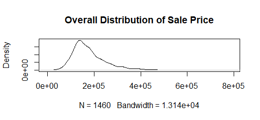
The next step in the data exploration was to look at the distribution of the different variables and to transform them as needed. The outcome or response variable, is the sale price of the home, which is a continuous variable, but with a marked right-ward skew.

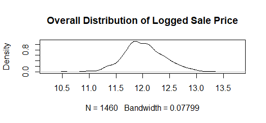
I therefore took the natural log of this variable in order to reduce the elasticity and make it appear more normal.

I also logged the other continuous variables such as area in square feet. The year variable was also treated as continuous, but instead of logging it, I transformed it to duration. That is, I got the number of years between the time the house was built to the time it was last sold as per the dataset, and the number of years between the time was remodeled to the time it was last sold.
I then examined the outliers in the continuous variables, and since I did not want to drop any observations, I reset them to the mean.
For all categorical variables, I examined the frequency distribution and the cell counts. Having a background in variance estimation, I am aware that cell-sizes of 1 are very problematic, and indeed small cell-sizes are in general problematic. I therefore combined categories where I could. For example, in terms of roof style, it would appear that gabled roofs are the most popular in Ames, and a majority of the homes (1141 out of 1460 in the train data) have gabled roofs.
The frequencies of other roof-styles are much smaller. I therefore combined all the other roof styles into one category, making the variable “Gabled Roof – yes or no”. Logically this seemed fine, since it would appear that either the market forces or building codes dictate the most common roof style. I did this for all categorical data types after examining their cell frequencies. If a variable had sufficient observations in each cell, I left it as multi-category variable.
Using Data to Analyze Missing values
Another set of categorical variables had large numbers of missing values to indicate the absence of the feature. For example, there were large numbers of missing values for basement, garage, fence, pool, and fireplace, to indicate that the house did not have these features. In such cases, I changed the missing values to zero to better indicate the absence of that feature.
There is a caveat here however. Basement had a number of different categorical variables to describe it. However, the missing values here were inconsistent, which indicated that at least some were true missings rather than indicating the absence of a basement. I therefore set to zero only those observations where all the basement variables were missing. Anything else was treated as a true missing. Other variables such masonry-veneer-type also had multiple true missings.
All true missing values across variables were imputed using KNN Impute.
Using Data to Analyze Additional feature selection
Once the variables were transformed, I ran them through a forward AIC model to further narrow down the number of variables to be included in the final models. In the end, I had selected 31 variables to include in the final regression models.
Using Data to Analyze Regression models used
To predict the sale price of a home, I ran various models, and checked to see which provided the best prediction. The models included the following:
- The ordinary least squares model (OLS)
- Ridge regression
- Lasso regression
- Elastic-Net regression
- Gradient Boosting regression
- Decision Tree regression
- Random Forest regression
All models, except the OLS were run using grid-search with a 10-fold cross-validation.
Results
I checked the model fit of each model using three metrics – the R-square, the Mean Square Error (MSE) and the Root Mean Square Error (RMSE). The best fit model would have the highest R-square, and the lowest MSE and RMSE.
Here’s what these metrics looked like for each model, along with the graph of the fit:
- OLS
- R-square of .889
- MSE of 0.017
- RMSE of 0.129

This model fits the data well, although there is some over and under-fitting at the extremes.
- Tuned Ridge:
- R-square of .870
- MSE of 0.017
- RMSE of 0.129

As with the OLS, this model fits the data fairly well, but again with some over and under-estimation at the extremes.
- Tuned Lasso:
- R-square of .821
- MSE of 0.027
- RMSE of 0.164

Unlike the OLS and Ridge models, this does not fit the data well at all.
- Tuned Elastic-Net
- R-square of .662
- MSE of 0.051
- RMSE of 0.226

The metrics and the graph show clearly that this is not a good model for predicting home prices with this set of variables.
- Gradient Boosting Regression:
- R-square of .842
- MSE of 0.020
- RMSE of 0.141

Although the metrics for the gradient boosting regression are not as good as the OLS and the Ridge regression, it nevertheless fits seems to fit the data very well.
- Decision Tree:
- R-square of .764
- MSE of 0.017
- RMSE of 0.129

The metrics for the decision-tree show that it does not fit the data well at all. However, the graph is as expected for a decision tree, and shows the clustering of the data at different nodes.
- Random Forest:
- R-square of .779
- MSE of 0.026
- RMSE of 0.129

The metrics and the graph both show that the random forest does not fit the data well at all. There is significant over and under-estimation of data points and not just at the extremes.
Models selected
Based on the metrics to determine the fit as well as the graphs, I chose the following models as being the best fit for the data:
- The OLS
- The Ridge regression
- The Gradient boosting regression
I submitted these to Kaggle for a score, and the OLS, which did in fact have the best fit of all the models, obtained the best score.
Concerns
From a variance estimation and traditional statistics perspective, there are a few issues to make a note of, though they matter less for prediction models.
- The clustering effect of the neighborhood variable.
- The significant spatial-autocorrelation in the dataset. This violates the assumptions of the OLS.
- The very large standard errors around the estimates in the OLS.
Admittedly, they matter less for prediction models, but nevertheless, it is important to be aware of these issues.
Conclusion
Overall, this was an interesting exercise, and one that really brought home to me the predictive power of the different machine learning models. In the future, I would like to run a support-vector machine regression on these data, and also try including the full feature set (appropriately transformed and adjusted).


