Using Data to Predict House Prices in Ames, Iowa
The skills the authors demonstrated here can be learned through taking Data Science with Machine Learning bootcamp with NYC Data Science Academy.
1. Introduction
Based on data, there are several factors involved with the sale price of a house. Some things that come to mind are size, number of bedrooms, year built, neighborhood, proximity to grocery store, etc.
In the Kaggle Competition: “House Prices: Advanced Regression Techniques” created by Dr. Dean De Cock, our team explored a multitude of variables to further understand what influences the value of a house and how we can use these variables to predict the sales price given specific characteristics.
The goals for this project were:
- Explore the data set and variable influences on sales price
- Address data missingness, skewness
- Feature engineer
- Deploy machine learning methods
2. Data Preprocessing
2.1 Data Exploration
The first thing after getting this dataset is to explore the data. This dataset contains all kinds of data type: numeric, ordinal, categorical and binomial.
2.2 Data Cleaning
-
Using Data to Analyze Finding Outliers
For finding outliers which decrease fitting performance of prediction model, We made assumptions that follows common sense. People usually consider Unit Price of houses. And they might listen to voice of the market, Overall Quality Ratings.
Commonly, these two variables have a proportional relationship. And the Unit Price will follows normal distribution by each rating. Anyone can think this. And we will check our given data follow these assumptions through this plot.
 Now, we can see distribution shapes of normal distribution by each rating and found little bit strange shaped distribution, rating 10. What happens in rating 10?
 -
Using Data to Analyze Handling Outliers
We checked all of data at rating 10. As results, 13 outliers were found. And we removed 2 outliers which are leverages in 9 variables. So, we could improve fitting slopes and R-squared coefficients (0.69 → 0.77) each variable. Below, this table is about improved slope value changes.
 And these plots describes examples of slope changes.
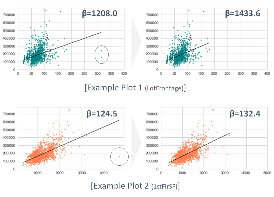
The R-squared values and betas are coefficients of slope from multi linear regression score. Actually, these value improvements are not directly related to result of this project. But, these will contribute to models in the prediction procedure. -
Using Data to Analyze Transformation
As one of the assumptions for linear regression, we checked normalities of all numerical variables. The test method was D’Agostino’s K-square test.
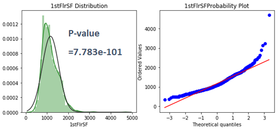
This variable doesn’t follow normal distribution. So, we transformed these by using logarithm, reciprocal, square root and reciprocal square root transformation method.

We transformed 10 explanatory variables and corrected their skewness and kurtosis. And not only explanatory variables, also target variable (SalePrice) could be corrected with log transformation method.
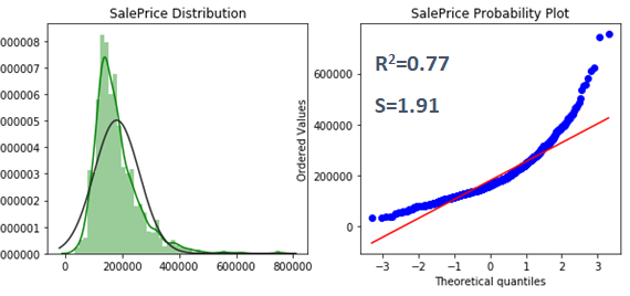
This plot describes positive direction skewness. We tried all methods for correcting this.

Finally, we could optimize the correction through log-transformation.

We can check the difference between before and after transformation. Original data looked like quadratic distribution on the red line. But, now it became nearly linear. That means this data follows normal distribution. Of course, after we finish predict from this dataset, we will change transformed target value by using exponential function.
2.3 Using Data to Analyze Missing Imputation (1/2)
The entire data set (training + test) has 34 variables with missing data, 13,965 values out of 115,340 values (12%). Some of the variables, such as ‘PoolQC’, ‘MscFeature’, ‘Alley’ and ‘Fence’, have more than 80% data missing. The imputation of those columns could be a huge challenge without any leads. The natural way is to find how the original data set says about those variables.
The data description has specific definitions for many of the ‘NA’s in the data set, for example, ‘NA’s in ‘Alley’ column simply indicates that there is no alley for the house, and ‘GarageArea’ would be ‘NA’ too if there is no garage in the house. Therefore, by looking at the data description, 15 categorical and 10 numerical features can be imputed by either ‘None’ or number 0, depending on the original data type of the feature.
After this round, we only have 34-25 = 9 columns left to be imputed. If we look at the numbers of the missing data among those features, 8 of them are only missing less than 4 values, which can be imputed by the most frequent values in their corresponding columns. Now, the only feature left here is ‘LotFrontage’, the linear feet of street connected to property.
Since there are 486 (17%) data missing, a cautious way to handle it is to use kNN to help determine the values, with the consideration of all other features, including ‘Neighborhood’ and ‘LandContour’ that may have bigger influence on the street around the house. However, in order to use kNN, we have to wait until all other categorical features to be properly converted (labeled) with numbers.
2.4 Using Data to Analyze Label Encoding
There are 79 features (36 numerical + 43 categorical). We examined each of them and divided them into 4 cases: A, B, C and D to handle them differently. Case A indicate 33 numeric features that do not need any further transformation. They are mainly area in square feet, or quality levels that are already in ordinal numbers.
Case B, however, are 3 numerical features that require closer look. By definition, ‘MSSubClass’ is using integer numbers to indicate certain house types. Therefore, they are actually categorical values. We converted this feature to categorical -> numerical by sorting out their corresponding average ‘SalePrice’. ‘SalePrice’ does not have monotonic dependence on ‘MoSold’ or ‘YrSold’ either. So we also converted them in a similar way as ‘MSSubClass’.
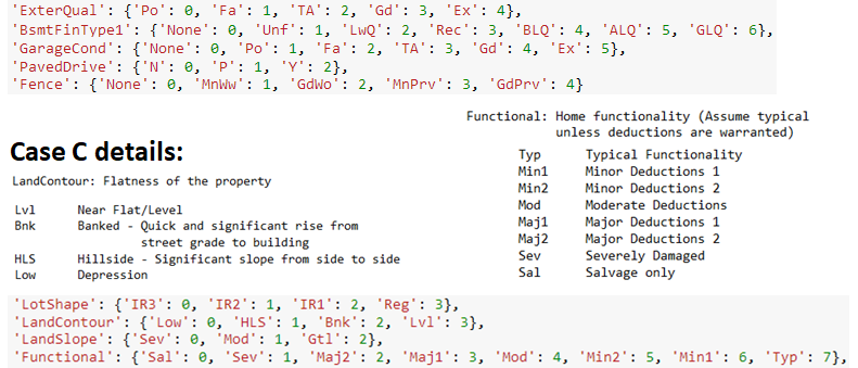
Case C consists 25 categorical features that are evaluating qualities or conditions. They can be intuitively labeled by ordinal integer numbers. Some of them, such as LandSlope’, ‘LandContour’ and ‘Functional’, are also showing specific trends regarding certain house conditions. So they were also labeled based on their direct meanings.
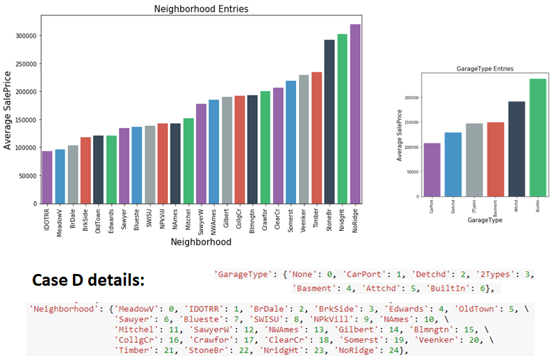
Case D includes the last 18 features with categorical values that are not showing obvious dependence with ‘SalePrice’ by the first look. For example, it is hard to tell how the ‘RoofMat1’, ‘GarageType’, ‘SaleType’ or ‘Neighborhood’ would influence the house price. Instead of ‘one-hot-labeling’ or ranking them based on value frequency, we again use their corresponding average ‘SalePrice’ to sort and give them integer labels as we did to Case B.
2.5 Using Data to Analyze Missing Imputation (2/2)
With all the other 78 columns filled and properly converted to numerical values, it is time to revisit the last column with missing data. We chose to use Manhattan distance to impute ‘LotFrontage’ to reflect more subtle details from other data points and to reduce the influence from larger distance dominating the imputation results. k-Neighbor = 5 was determined by the R^2 resulted by a series tests of k numbers.
3. Using Data to Analyze Modeling
3.1 Using Data to Analyze Base Models
Three linear models were tested and used to predicted on the training data. While Ridge Regression tend to keep all the 79 features, Lasso Regression dropped 24 features as unimportant. After the grid search Elastic Net Regression consisted 91% of Lasso. In all cases the ‘OverallQual’, ‘OverallCond’ and ‘GrLivArea’ are the three features that show most import positive influences on the ‘SalePrice’.
Besides linear models, two tree models, Gradient Boosting and Random Forest, as well as a non-linear model, Kernel Ridge Regression were also tested and used for house price prediction. The corresponding training error and Kaggle Public Board error are shown below.
The training and PB errors show that overall our Gradient Boosting and Kernel Ridge models are making the best prediction, linear models show slightly larger errors, and that the Random Forest model produces largest errors. Therefore we chose Gradient Boosting (GBoost), Elastic Net (ENet) and Kernel Ridge (KRR) Regression for further model stacking.
Before running into model stacking, we examined the actual comparison between the predicted and true ‘SalePrice’ values along the y = x line for our three best models. ENet and KRR show similar data distribution features despite the fact that ENet has bigger errors at high price region, mainly because they are both using l2-squared error in the loss function. One of the main sources of our linear models is rooted in the multicollinearity: We didn’t combine strongly correlated living/basement area features.
Comparing with the other two, GBoost did better overall predictions, but it still made several predictions that are far deviated from the y = x line. Therefore, further model stacking is needed to help adjust the differences between models to give more accurate results. A simple averaging between the predicted ‘SalePrice’ among three models has already reduce the training and PB error significantly.
3.2 Using Data to Analyze Model Stacking & Ensembling
Our stacking approach followed simple “greedy manner”. Since we only have three starting models, there are only three choices for the meta-model when picking two as bases. Our results shows that the meta-model of ENet trained by stacking GBoost & KRR gave the lowest errors, which are lower than the simple averaging results.
For the model ensembling, we again apply the greedy forward approach: picking up the best model, linear Lasso Regression among other candidates. With a simple ensembling formula of 3 quarters of meta-model + 1 quarter of Lasso, our final RMSLE PB error was further lowered down to 0.11718, among the top 600 results.
4. Future Works
Since the main source of our linear models came from multicollinearity, our future improvement in the data pre-processing part will be including:
- Combining different group features, especially those involving aspects with living / basement / garage areas
- The skewness transformation can be performed after feature engineering;
Different skewness transformation methods for both features and target columns can be used besides Box-Cox and Log.
Meanwhile, for the modeling part:
- More diverse or advanced/efficient machine learning models can be included, such as XGB, LightGBM, PCA…
- Based more models and improved results, more stacking & ensembling combinations can be tested to further lower down the errors.
References & Useful Links
For more information, welcome to visit our group GitHub to find more details. We also thank Kaggle Kernel authors for useful EDA and modeling insights for the dataset.


