Using Data to Predict Housing Sales Prices in Ames, Iowa
The skills the authors demonstrated here can be learned through taking Data Science with Machine Learning bootcamp with NYC Data Science Academy.
Sangwoo Lee, Shailendra Dhondiyal
Introduction
In this research, we investigated factors influencing sales prices of houses. We used a Kaggle data set consisting of information on 1460 home sales in Ames, Iowa between 2006 and 2010. After studying 79 input features and the basic characteristics of the data set, we built regression models for the sales prices by applying Python machine learning algorithms. We also tried to uncover the key drivers of the sales prices. We think that these modeling efforts can help not only businesses but also individuals in optimal pricing and in identifying key features influencing house sale prices.
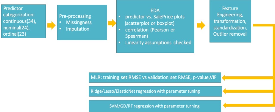
The overall procedure of our research is summarised in Fig. 1.
Fig. 1 Overall procedure for data processing through performance evaluations
Data Processing
Handling Missing Data
Many features showed a high number of NaN. But on checking the data descriptions, we found NA for a number of features when they were not present in the house. We replaced missing values in such cases with 0 as per our understanding, whether the given number can be of such houses. For other missing data, we appropriately imputed or dropped, as in Table 1.
 |
Table 1. Missing data handling methods
Data Processing Per Feature Types
We categorized 79 input features to 33 continuous, 23 nominal, and 23 ordinal features. Values of ordinal variables were replaced by integers as per order. For instance, BsmtCond feature was expressed by 1,2,3,4 and 5, respectively meaning poor, fair, typical, good, and excellent.
As for nominal features, instead of using dummification methods, we ordinalized the features. As an example, as shown in Fig. 2, on a boxplot showing the relationship between the Neighborhood feature values and the SalePrice, we grouped the Neighborhood feature values by the medians of the SalePrice.
 |
Fig. 2. An ordinalization example of nominal predictor ‘neighborhood’
Exploratory Data Analysis
We checked EDA in several aspects. We checked continuous features’ linearity with log(SalePrice) graphically by scatterplots and computationally by finding Pearson correlations, as in Fig. 3a). For nominal and ordinal features, boxplots with log(SalePrice) and Spearman correlation values were checked, as in Fig. 3b) ~ 3c). We also ascertained whether or not fundamental assumptions underlying linear regressions are met, as in Fig. 4. By confirming that linearity assumptions are valid for this modeling, we could find that multiple linear regression models can be applied as the starting point of this research.
 |
a) EDA of log(SalePrice) linearity with continuous predictors. Pearson cross-correlation between log(SalePrice) vs. continuous predictors was also checked.
 |
b) EDA of boxplots between nominal predictors and log(SalePrice). Spearman’s cross-correlation between log(SalePrice) and nominal predictors was also checked.
 |
c) EDA of boxplots between ordinal predictors and log(SalePrice). Spearman’s cross-correlation between log(SalePrice) and ordinal predictors was also checked.
Fig. 3 EDA of continuous/nominal/ordinal predictors
|
a) Normal distribution of response variable |
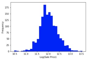
b) Log transformation of ‘SalePrice’ to address skew to right |
|
c) Normal distribution of residuals checked |
d) Constant variation and auto-correlation |
Fig. 4 Assumptions of linear regression verified ( Linear relationship between the response variable and the independent variables were checked in terms of correlation and scatterplots as in Fig. 3 )
Short listing the Features
For modeling and performance evaluations, we decided to shortlist the features on the basis of a correlation threshold of 0.4 (moderate and above, either Pearson or Spearman correlations) with log(SalePrice). After shortlisting, we arrived at a reduced data set with 27 features and 1 response variable. We started from this shortlisted data set, and iteratively searched for data sets which yielded better results in MLR(multiple linear regressions) first.
Results
In Table 2, we compare performance of different linear/non-linear machine learning algorithms. We aimed at lowering the RMSE(square root mean square error) between true log(SalePrice) and predicted log(SalePrice) on the validation fold as much as possible.
In No 1 ~ No 4, we compared linear modelling algorithms such as MLR(Multiple Linear Regression), RR(Ridge Regression), LR(Lasso Regression), and ENR(ElasticNet Regression). After starting from correlation threshold 0.4 for feature shortlisting,and through trial-and-error, we realized that adopting a correlation threshold of 0.3 for 41 input features, in fact, produces better results. Using the correlation threshold 0l4m, we obtained 0.123 on the validation fold for No 1 ~ No 4. When RR results of No 2 were further extended and submitted to the Kaggle website, we achieved a Kaggle score of 0.13741.
We picked GDR(Gradient Boosting Regression), a non-linear algorithm with less complexity than RFR(random forest regression) but with performance similar to that of RFR, as a comparison case. After further feature selections for finding good GDR performance, we realized that allowing a full set of continuous/ordinal features for GDR improves performance. As in No 5 of Table 2 below, we obtained RMSE of 0.120 on the validation fold, and a Kaggle score of 0.1315.
 |
Table 2. Modeling Results
In Fig. 5, Feature Importance as per random forest modeling is provided.
 |
Fig. 5. Feature Importance as per Random Forest
Conclusions
From feature selection points, we found several points. First, as expected, area is a key driver of prices. Second, while having a garage is important, its qualityis not so important. Thirdly, contrary to expectations, MSSubClass (type of dwelling) and MSZoning (general zoning classification) did not come out as important features. Lastly, Fireplace – both quality and availability – which might be low cost features, are valued
For further studies, we think that more work is needed for dummification of nominal and ordinal variables, and application of domain understanding in combining variables. As for model designs, applying Principal Component Analysis to generate features and then doing regression with key features can further enhance performance.


