Heat Sink Surface Defect Detection with Image Segmentation

Introduction

Smart Manufacturing and Defect Detection

The entire landscape of the manufacturing industry has been transformed for the better with the advent and precipitous implementation of Smart Manufacturing. The integration of modern information technology, notably big data and AI capabilities, has drastically increased manufacturing productivity and brought along many other benefits including the optimization of resources, predictive maintenance and reduction in manpower processes.

Quality control is undoubtedly one of the most important aspects of any manufacturing process. It is critical to ensure only parts that meet specification and do not have unacceptable defects make it to the customer since the reputation of a manufacturer is largely staked on the quality of their products. Traditionally, quality inspection could consist of operators or technicians visually checking parts for defects under a microscope, picking out faulty parts and perhaps keeping records of the failed parts as well as some details regardings the defects. One of the components of smart manufacturing is the automation of quality inspection using deep learning based computer vision. The successful implementation of this technolgy can bring about many benefits including but not limited to the list below:

• Reduction in human labor - Cameras and machine learning algorithms can replace operators and technicians in inspecting the parts for defects and filtering the passes/fails.
• Increased efficiency - Using cameras and machine learning algorithms is likely able to conduct quality inspection faster than humans. Machines and computers are also not restricted to usual working hours and do not require rest, meaning manufacturing can occur for as long as need without down time.
• Potential improvement in accuracy and consistency - It is impossible for humans to remain focused for an indefinite amount of time and can inadvertently become careless or miss certain details. Human judgement can also vary from person to person so if there is any room for ambiguity in terms of failure criteria, quality control can become inconsistent. With computer algorithms, the result would always be reproducible.
• In-process quality control - With smart manufacturing, it is possible to incorporate quality inspection seamlessly into any and all stages of the production line since all that's needed is perhaps a camera and some mechanism to filter the defective parts. For manual inspection, it might be necessary to set up separate inspection stations onto which parts have to be transferred which can greatly obstruct the workflow, let alone the resources that would need to be dedicated to those extra stations. It would also require an extremely large amount of manpower to have quality inspect after every manufacturing step. Having quality inspection after every manufacturing step is desirable since faulty parts should be removed from the production process as soon as possible to avoid using up any more resources down the line.
• Data-based failure analysis and process improvement - With computer vision, a very large amount of data as well as intricate details regarding the parts can be recorded. Having the data would be extremely valuable in determining root causes for failures and finding weaknesses or bottlenecks within the process.

Project Description

The goal of this project is to use deep learning to detect defects on heat sink surfaces, in a way that could be realistically be implemented in the industry.

Data Description

The dataset can be found on Kaggle: https://www.kaggle.com/datasets/kaifengyang/heat-sink-surface-defect-dataset.

Citation for the originally published paper on the dataset: K. Yang, Y. Liu, S. Zhang and J. Cao, "Surface Defect Detection of Heat Sink Based on Lightweight Fully Convolutional Network," in IEEE Transactions on Instrumentation and Measurement, vol. 71, pp. 1-12, 2022, Art no. 2512912, doi: 10.1109/TIM.2022.3188033.

The data is collected and labeled by State Key Laboratories of Transducer Technology, Institute of Semiconductors, Chinese Academy of Sciences.

The dataset contains 1000 images of gold-plated tungsten-copper alloy heat sink surfaces, with defects and their annotations.

The images are labeled into categories:

• 0 - Backgroud (defect-free area)
• 1 - Scratch
• 2 - Stain

An example image (original and labeled) can be seen below.

Data Exploration

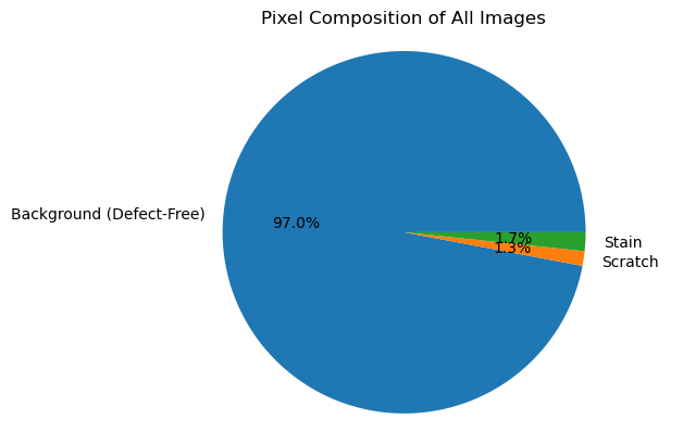
In terms of pixel composition of all images, most of the area is by far the background. Stains and scratches only account for 1.7% and 1.3% of all pixels, respectively. This could be concerning as the target classes are so dispropordispropotionate and the defects constitute such a small portion of all pixels. It also means that even if the model predicts all pixels as the background it would have an accuracy of 97% already which gives a false illusion of how well the model performs.

Of the 1000 images, every image has labeled defects. 28 images only have scratch. 300 images only have stain. 672 images have both scratch and stain. Around 2/3 of all images have both scratches and stains.

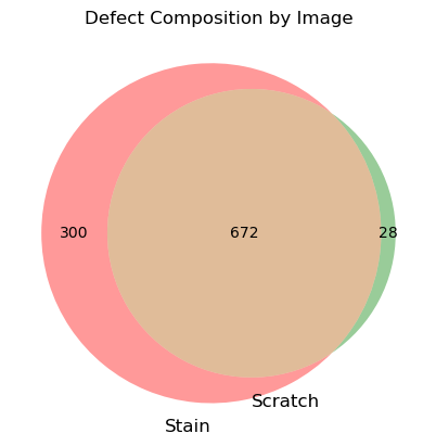
Image Segmentation with U-net CNN

Data Preparation

Split data into 70/15/15 Train/Validation/Test sets.

Preprocess data by resizing images from 320×320 to 256×256 and normalizing input values by dividing RGB values by 255.

U-net Implementation

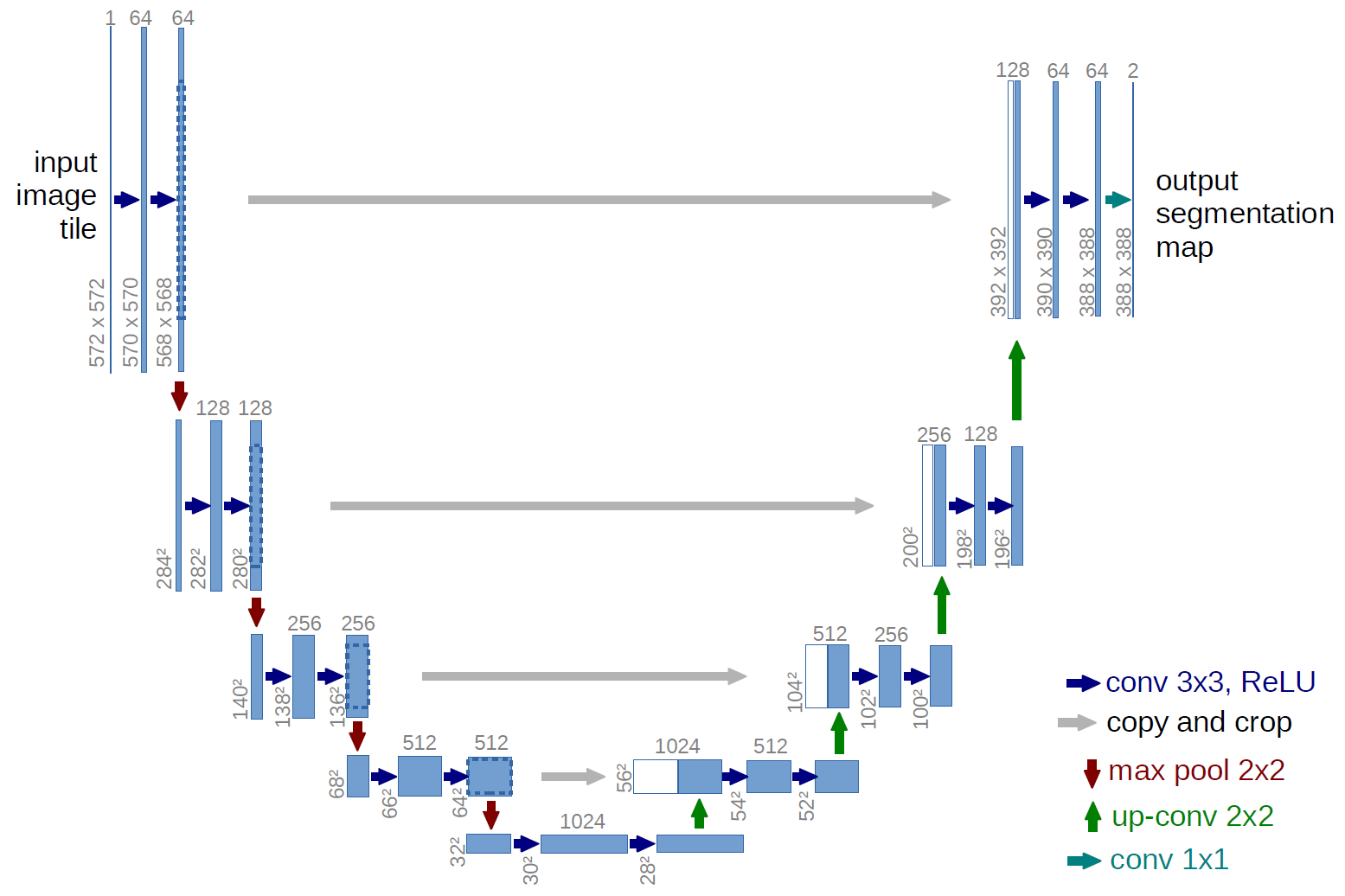
The original U-net architecture can be found below.

Ronneberger, O., Fischer, P., Brox, T. (2015). U-Net: Convolutional Networks for Biomedical Image Segmentation. In: Navab, N., Hornegger, J., Wells, W., Frangi, A. (eds) Medical Image Computing and Computer-Assisted Intervention – MICCAI 2015. MICCAI 2015. Lecture Notes in Computer Science(), vol 9351. Springer, Cham. https://doi.org/10.1007/978-3-319-24574-4_28

For this project, the original U-net architecture was followed but the number of filters at each convolutional layer was halved to reduce the computational load, i.e first two convolutional layers have 32 filters instead of 64, subsequent two convolutional layers have 64, so on. Based on the architecture, skip connections in contracting blocks are tracked and concatenated to corresponding upsampling blocks. Also did not add any batch normalization or dropout. For training, batch size of 32 was used and trained for 40 epochs.

Results

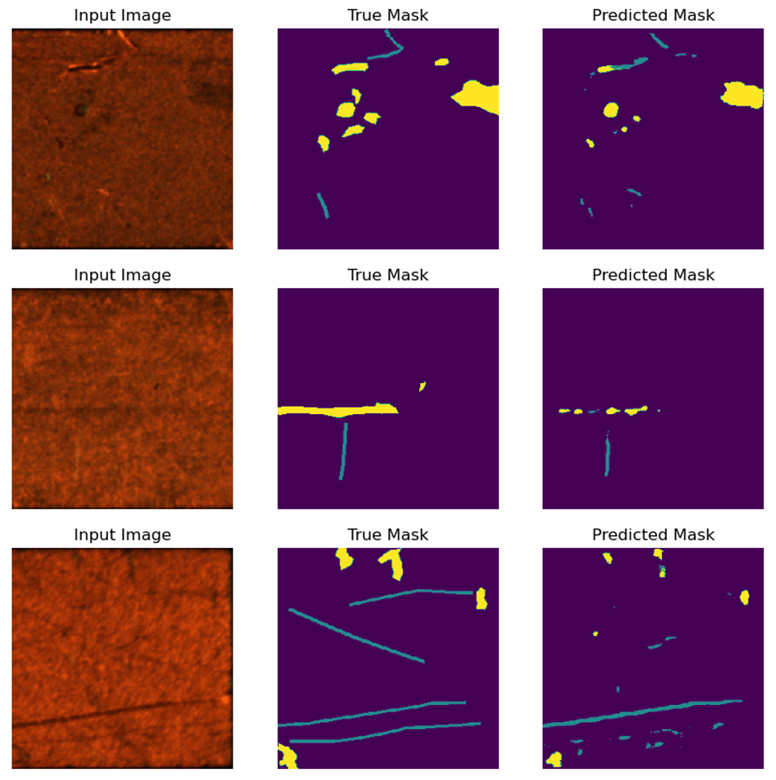
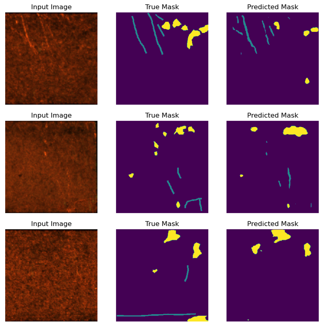
Using the trained model, a few examples of the training and validation set predictions can be seen below.

Training Set

Validation Set

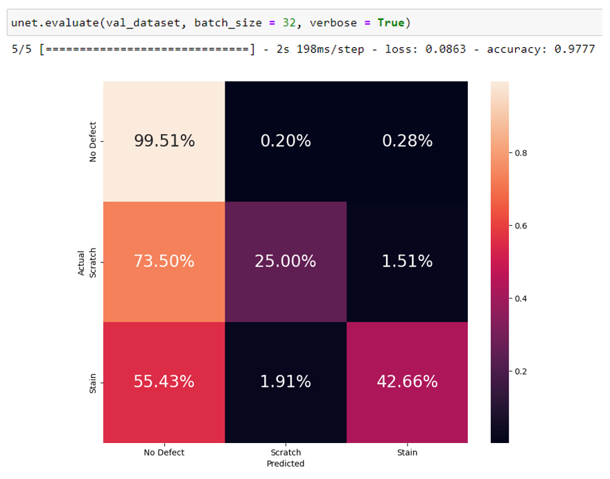
The pixel-wise confusion matrix for the validation set can be seen below.

As shown in both the example predictions and the confusion matrix, the model tends to over-predict the background (no defect area) over the defects. This is somewhat expected due to how disproportionately more the background is compared to the defects. The model is only able to correctly label 25% of scratches and 43% of stains which is rather low.

To investigate into how and why the defects are mislabeled, some examples are shown below where the types of defects predicted do not match the real mask. Examples of defect type mismatch could be the predicted mask has background and stains only but the real mask has background and scratches only, or predicted mask has background and stains only but the real mask contains all three classes.

Discussion on Labeling of Dataset

After checking many examples such as the ones from the previous section, it became apparent that the labeling of the defects is quite arbitrary as the criteria for each defects are not very clear at all. In most instances, it is difficult to judge whether a defect is present and also to discern whether or not the defect is a scratch or a stain. This indicates that the Bayes error and the human-level error for the task is inevitably quite high.

There are also many instances of unlabeled and mislabeled defects. In the example below, the circled defect should probably have been labeled as a stain (as the machine learning algorithm has) since it does not look very different from the other stains labeled in the image.

The example below shows an example of mislabeling. It is clear that the four images are taken next to each other but somehow the defect that spans across them is not labeled consistently.

The machine learning algorithm can only be as good as the quality of the training data allows it to be. Thus, given the inherently highly arbitrary nature of the defect labeling as well as relatively common mislabeling of defects, the ceiling for the algorithm performance is likely quite low.

Resnet50 and Vgg16 Backbone

Segmentation Models library allows for implementation of other architectures as the backbone for U-net (the encoding portion). The package also produces the decoding portion automatically for the user. All backbones have weights trained on 2012 ILSVRC ImageNet so transfer learning is utilized in this case.

In terms of model training, had to use batch size of 16 due to hardware memory limitations and trained for 40 epochs.

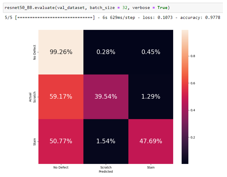
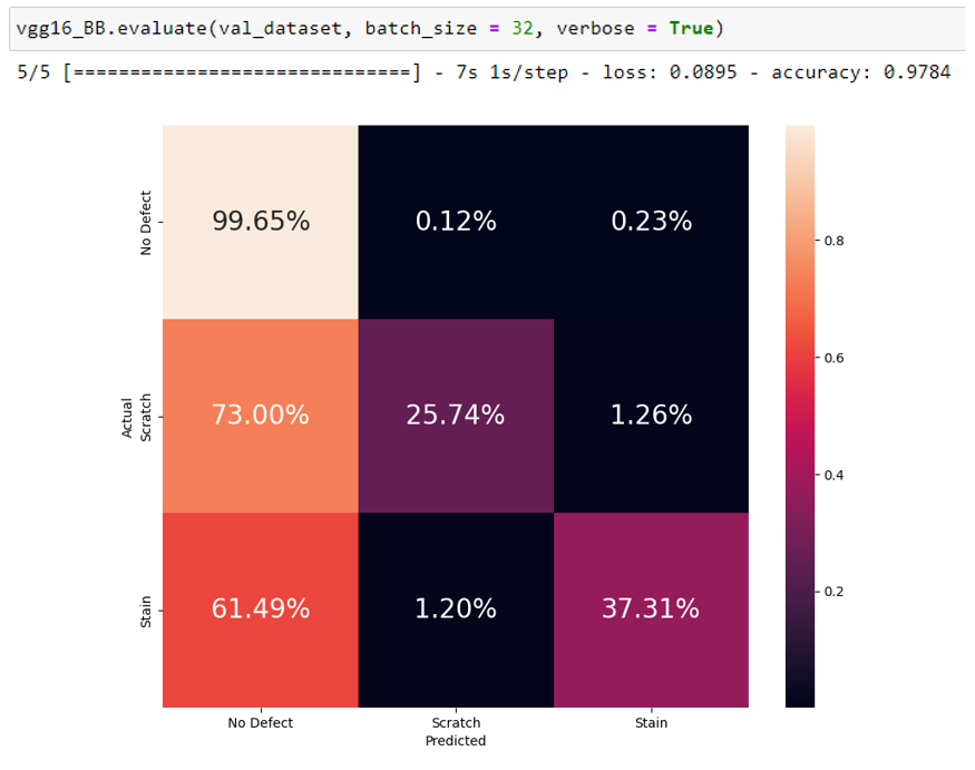
Below shows the validation set evaluation comparison between the three models.

Original U-net (Copy-paste of results from previous section)

Resnet50 Backbone

Vgg16 Backbone

The accuracies between the three models are all quite close at ~97.8%. It is important to recall that since 97% of all pixels in the true masks were labeled as the background, an accuracy of at least 97% should be expected as the baseline. While the Vgg16 backbone model had the highest accuracy of the three by a very small margin, the Resnet50 backbone model actually had the highest percentage of correct predictions for the defects at 40% of scratches and 48% of stains. Subsequently, the Resnet50 backbone model also had the lowest percentages of defects mislabeled as the background.

Some examples predicted with the three models can be seen below. As suggested by the confusion matrices, it should be the case that Resnet50 backbone model tends to be able to identify defects that the other two can not. This can indeed be seen in the circled defects which are only present in the Resnet50 backbone predictions.

Predicting Test Set

After evaluating the validation set results from the three models, it was decided that the Resnet50 backbone model would be the best choice as generally from a manufacturing business perspective, it is much better to overkill in terms of failures than to let defective parts slip through to the customer. Will proceed to apply the Restnet50 backbone model on the test set to confirm that performance is relatively consistent with that from the validation set and that there are no unexpected issues with implementation. The resulting confusion matrix and some prediction examples can be seen below.

Compared to the validation set, the model had slightly lower accuracy in terms of scratches and slightly higher accuracy for stains with the test set. The model appears to work decently well and the percentage of correctly labeled defects is still higher than that of the other two models for both defect types.

Post-Segmentation Image Analysis

After doing image segmentation, it is now possible to use the results to screen defective parts if there are established criteria.

Focusing on stains, change predicted masks to greyscale with only stains and background pixels. Use OpenCV to locate contours (stains), calculate areas, add minimum enclosing circles and locate their centers. The following table (sorted by LargestStainArea) can be produced and kept in record for future analysis.

Column Descriptions:

NumberOfStains - The number of detected stains.

LargestStainArea - The area of the largest stain calculated by OpenCV using the Green formula. Can be converted to actual size if the image scale is known.

LargestStainRadius - The radius of the enclosing circle for the largest stain.

EnclosingCircleX/Y - The X and Y coordinates of the enclosing circle for the largest stain, with (0, 0) being the top left corner of the image.

TotalStain% - The percent of pixels in the image that are stains.

Images below are #77 and #110 from the table above (2nd and 3rd row) and they help illustrate the OpenCV image processing.

With this functionality, it is possible to filter out faulty parts in the manufacturing process if there are established specifications such as an upper limit to the area of any given stain or the number of stains. This can also be used to monitor process quality and incorporate statistical process control. For instance, the size of the largest stain can be tracked in real time in a run chart and alerts can be set up for outliers or if the running average starts drifting out of specification range. Having collected all the data can also help in conducting failure analysis and pinpoint processes contributing to failure rate. For instance, perhaps it could be observed that the location of the largest stain is consistently at one corner of the part. Having knowledge of this pattern can help engineers trace back and investigate some part of the manufacturing equipment that comes into contact with the part at that location. Another use case can be studying the increase in the number of stains after every process and determining which process contributes to producing stains the most.

Conclusion

This project demonstrated the successful implementation of a defect detection program that could be used under a manufacturing environment to replace visual inspection done by operators or technicians. Image segmentation was performed on images of heat sink surfaces to detect defects including scratches and stains.

Implemented U-net CNN architecture as well as Resnet and VGG as backbones with pre-trained weights using Segmentation Models library. Of the three models evaluated, the Resnet50 backbone architecture was selected to be the best performing considering the nature of the task. There is a very large discrepancy in the distribution of target classes in that only 3% of all pixels are labeled as defects. The labeling of the defects is also very arbitrary and there exists quite a few cases of mislabeling. These factors preclude the model from attaining truly high accuracy.

Post-process analysis with OpenCV allowed for the determination of defect count, size and location. Results can be used to label and filter defective parts, monitor process quality, incorporate statistical process control, conduct failure analysis and pinpoint processes that contribute to defect rate.

Future Work

• Can perhaps incorporate some data augmentation such as image rotation, flipping, etc., to increase dataset size.
• Correct mislabeled cases or have better defined criteria for determining if defect is present and which type.
• Can try other achitectures and see if performance improves. Can also train for longer.
• For scratches, can implement rotated bounding rectangle and determine the length of the longer side as an estimate for the length of the scratch. This can be useful if there is specification regarding the maximum scratch length.
• If it can be known which pictures come from any given part, then can study the location and size of defects to see if there is pattern. For instance maybe top right corner of part is always scratched, and maybe this can be traced back to an issue with the equipment.

Project on GitHub