Advanced Regression Modeling on House Prices
Introduction
The key question addressed in this blog is how we can better predict the sale prices of residential houses. The Ames Housing Price data set recently released on Kaggle is “a modernized and expanded version of the often cited Boston Housing dataset”. It covers all the recorded house sale price in Ames, IA from January 2006 to July 2010. With 79 explanatory variables describing almost every feature of residential homes, we aimed to apply data imputation, feature engineering and machine learning modeling to achieve a better predictive accuracy on the housing price.
The dataset contains 1460 observations in the training set and 1459 observations in the test set. There are 46 categorical variables including 23 nominal and 23 ordinal ones, and 33 numeric variables in the dataset. The training set also has the sale price as response while the test set doesn’t.
Time Series
It’s important to note that the housing price data ranges from early-2006 to mid-2010. We should be aware that the subprime mortgage crisis happened during this period and contributed to the economic recession of December 2007 and June 2009. We drew the time series plot of monthly median house sale price below and decomposed the time series into trend and seasonality. As shown in the trend panel below, it’s obvious that the monthly median sale price had decreased steadily from early 2008 until late 2009. That would indicate the house sales in Ames was no exception and was influenced by the mortgage crisis. We derived the trend index and seasonality index from the time series. Since the time series for sale price appears to follow a multiplicative way such that Sale Price = Trend * Seasonality * Cyclicality * Irregularity, we calculated the time series index:
TsIdx = TrendIdx * SeasonIdx / max(TrendIdx).
We considered using those three time series indices as predictors to test if global economy could help predict the housing sale price.
Exploratory Data Analysis
Below are boxplots of some categorical variables vs sale price. They show consistency with our common sense that neighborhood, zoning, house quality and facility might distinguish the house value.
Scatterplots of some numeric variables are shown below. Some area related features such as lot area, 1st floor square feet, 2nd floor square feet, and house year built show positive correlations with sale price.
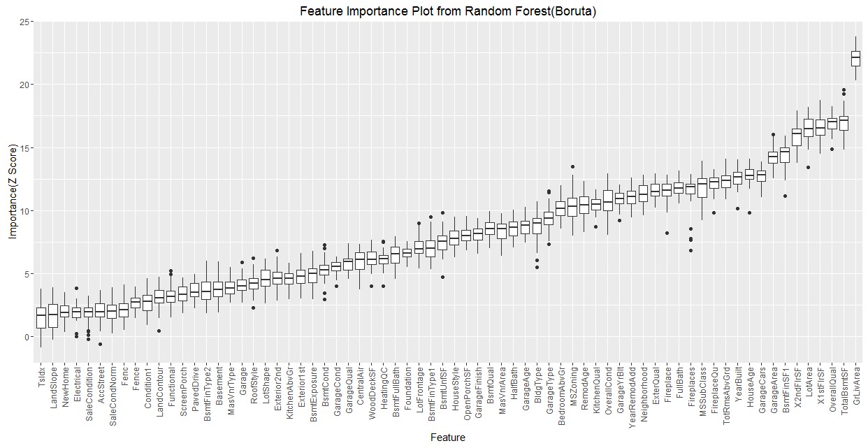
Feature Importance
Outliers
Modeling
We divided our modeling onto two sections. On the one side we modeled to achieve high predictive accuracy, and on the other side we modeled to maintain interpretation. We first discuss modeling that focused on achieving high predictive accuracy. As a first step we tuned parameters of all our base learners. We used grid-search to find the optimal parameters. Below are all the optimal parameters for our Generalized Linear Model, Neural Network, Random Forest and Gradient Boosted Trees .
GLM
Neural Network
Random Forest
Gradient Boosted Trees
Stacking
Next we used ensemble learning to combine our models. Ensemble machine learning methods use multiple learning algorithms to obtain better predictive performance than could be obtained from any of the constituent learning algorithms. Stacking is a broad class of algorithms that involves training a second-level "metalearner" to ensemble a group of base learners. The type of ensemble learning implemented in H2O is called "super learning", "stacked regression" or "stacking." Unlike bagging and boosting, the goal in stacking is to ensemble strong, diverse sets of learners together. In order to train the ensemble we did the following.
- Trained each of the L base algorithms on the training set.
- Performed k-fold cross-validation on each of these learners and collected the cross-validated predicted values from each of the L algorithms.
- Combined the N cross-validated predicted values from each of the L algorithms to form a new N x L matrix. This matrix, along with the original response vector, is called the "level-one" data.
- Trained the metalearning algorithm on the level-one data.
- Used the "ensemble model" consisting of the L base learning models and the metalearning model, to generate predictions on a test set.
Model Averaging
Stacking did not give us the intended results, although it improved our score slightly and did put us in the top 20% of participants. We therefore decided to use model averaging. This is a simple strategy where you average out your predictions. Below is a simple visual representation.
Seeing as this approach gave us significantly better results, we decided to include even more models into the averaging, placing more weight on the models we know performed well.
This approach pushed up to number two in the leader board on Kaggle.


