Analyzing Data to Predict House Prices in Ames, Iowa
The skills the author demoed here can be learned through taking Data Science with Machine Learning bootcamp with NYC Data Science Academy.
Introduction
Selling a home can be a daunting task and it is often difficult to estimate exactly how much value to place on a home given a particular set of features. Many homeowners decide to renovate their home to increase the value and attract prospective buyers. In this project, using a dataset from Kaggle.com, we answer two research questions: first, how accurately can we predict sales prices for homes using data from regularized linear regression models and tree-based models, and second, which changeable features are most important for a homeowner looking to add value to a home?
Background
The dataset contains 79 features describing 1460 individual houses in homes in Ames, Iowa between the years 2006-2010. This dataset is part of one of the most popular contests on Kaggle involving the usage of advanced regression techniques to predict housing prices and is often a starting point for novice data scientists and machine learning practitioners.
Exploratory Data Analysis and Processing
Linear Models
Since we planned to use a regularized linear model, we first checked the 4 linear assumptions on our dependent variable. The target variable, SalePrice, did not pass the initial test of normality. After applying a log transformation, our data passed all assumptions.


Findings
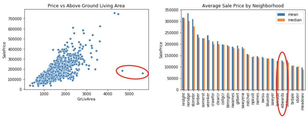
We encountered two apparent outliers when viewing plots of various features with house price. The outliers can be seen on the graph below.

After isolating these two home sales in the dataset, we found a peculiar backstory that led us to decide to drop them from the dataset. First, they were the two biggest houses in the dataset, both with the highest possible scores on Overall Condition and Quality, built in 2007 and 2008 respectively. They were both built in the Edwards neighborhood, which was fifth-lowest in terms of median sale price. And finally, both were partial sales.
Connecting the dots, we can see that these were speculative home builds from the peak of the housing bubble, and as the market turned downwards, the sale price seemed to reflect the neighborhood more than the size or condition of the home. After testing our models with and without these outliers, we found they skewed our results and we decided to remove them from consideration.
Correlation Plots
Finishing up EDA, we created two different correlation plots to get a feel for the most relevant features in the dataset. First, we created a correlation matrix to get a sense of multicollinearity between features. We found some features with high correlation, such as GarageArea and GarageCars. This makes sense because these two features essentially measure the same space in different units (square feet vs number of cars). In our Multiple Linear Regression model to come, we would have to choose between one or the other in order to ensure a stable model.
Numerical Feature and SalePrice
Next, we plotted the correlation between our numerical features and SalePrice in order to identify which of these features seemed to have the greatest impact on SalePrice. The top three were Overall Quality, Above Ground Living Area, and Exterior Quality. This gave us an idea of which features to look out for in the models to come. If we did not see these and the other highly correlated features stand out in our machine learning models, we would want to further investigate why.

Right: Correlation between Sale Price and numeric features
To test the significance of the categorical features, we ran ANOVA tests between each of these features and SalePrice. This revealed that all except Utilities were significant, so we excluded Utilities from our final models.
Machine Learning Models Data
1. Lasso
We implemented several machine learning models for several different purposes, starting with a Lasso model for the purpose of empirical feature selection. Then we created two predictive models, one linear (Elastic Net) and one non-linear (Random Forest). Finally, we ran an interpretive Multiple Linear Regression to find which features make for the most impactful renovations.
Lasso favors less complicated models by introducing a penalty term on predictor coefficients, which gradually approach zero as the penalty term increases. By choosing the appropriate penalty strength (decided by the hyperparameter lambda), certain predictor coefficients would be sent to zero while others remained non-zero, and predictors highly correlated with other predictors would have their overall impact regulated. Therefore, we could obtain a shortlist of important predictors and take care of the multicollinearity problem between them.
Through grid search with cross-validation, we selected the Lasso model that fit the dataset well without overfitting (shown at the crossover point between Validation Score and Train Score in the plot below). This model reduced the number of predictors from the original 224 (including dummy variables) down to 87. Among them, numerical variables that showed a high correlation with (log) SalePrice, such as Overall Quality, Garage Cars, and Above Ground Living Area, were included, as well as categorical variables that indicated Neighborhoods, Roof Material, etc.

2. Elastic Net
With the selected features from Lasso, we ran an Elastic Net model for the purposes for predicting Sale Price. Using grid search and cross-validation, we again chose parameters that fit well without overfitting. Our best parameters were Lambda = 1e-6 and L1 Ratio = 1.0. It is worth noting here that since our best L1 Ratio for Elastic Net was 1.0, it ended up behaving just like a Lasso model; but the grid search on Elastic Net allowed us to test the whole range of L1 Ratios before deciding that 1.0 was our best option. We’ll break down our scores below.
3. Random Forest
We selected random forest as our non-linear predictive model since it is a well-tested tree-based model that is generally robust to overfitting. Our model performed significantly worse than the linear regularized models, with a drop of almost 0.10 in the test score from Elastic Net. The decline in performance using a non-linear model on this dataset may be attributed to the fact that house prices seem to have an intrinsic linearity. Intuitively, the value of a house will typically increase as features are added or improved. The value will decrease as features are removed or depreciated. This natural linearity allows for linear models to perform very well on our dataset.
As we can see in the charts below, the linear Elastic Net model performed better than the non-linear Random Forest model, indicating that the (log) price of a house has a linear relationship with its features.

4. Multiple Linear Regression
Our final machine learning model was a Multiple Linear Regression on a particular subset of predictors built to answer the following question: what can a homeowner do to increase the value of their property? In other words, if a homeowner wanted to make some renovations, which ones would have the greatest impact on Sale Price?
The reason we chose Multiple Linear Regression was for interpretability, and the simple story that its coefficients tell. In a Multiple Linear Regression, for every 1 unit increase in a given feature, you can expect the target variable to increase by the value of that feature’s coefficient. This allows for easy interpretation, and therefore straightforward insight for homeowners.
Features
To choose our features for this Home Improvement Model, we started with the list of 87 features provided by our Lasso model. Because Lasso is nothing more than penalized linear regression, it makes sense to use Lasso’s output features as MLR’s input features. Next, we narrowed the feature list to only those that a homeowner has the power to change. For example, you can’t change your property’s neighborhood, so those were excluded. But you can change the quality of your kitchen and the pavement of your driveway, so those kinds of features were included. In the end, we kept 30 features for this model.
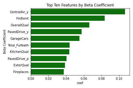
The model earned a train score of .881, giving us confidence in the model’s ability to explain the data, and ultimately its choices for most important features. After sorting the feature coefficients in descending order, we found the following to be most important.

Findings
We would hope that when deciding which renovations to make, a homeowner in Ames, Iowa might choose from this list. It might be difficult to install central AC, but we found that doing so would have the highest impact on value. For a simpler renovation, they could increase the finished percentage of their basement. This was our second-highest ranking feature, and could attract buyers willing to spend more for a fully finished property. Or for the simplest renovation of all, they could fully pave their driveway. That was the fourth-highest ranking renovation, and with the right tools it’s one that could be done on a long weekend.
Conclusion
In summary, we aimed at answering two main questions in this project: will the regularized linear or tree-based model better predict house price of the given dataset? And what changeable features are most important for a homeowner who is looking to add value to a home. Our analysis showed that a regularized linear model (Elastic Net) makes better predictions than a tree-based model (Random Forest), and we were able to get a list of features ranked by value importance for homeowners looking to add value to their property with renovations.

