A Data Scientist's Guide to Predicting Housing Prices in Russia

Sberbank Russian Housing Market

A Kaggle Competition on Predicting Realty Price in Russia

Written by Haseeb Durrani, Chen Trilnik, and Jack Yip

Introduction

In May 2017, Sberbank, Russia’s oldest and largest bank, challenged data scientists on Kaggle to come up with the best machine learning models to estimate housing prices for its customers, which includes consumers and developers looking to buy, invest in, or rent properties. This blog post outlines the end-to-end process of how we went about tackling this challenge.

About the Data

The datasets provided consist of a training set, a test set, and a file containing historical macroeconomic metrics.

• The training set contains ~21K realty transactions spanning from August 2011 to June 2015 along with information specific to the property. This set also includes the price at which the property was sold for.
• The test set contains ~7K realty transactions spanning from July 2015 to May 2016 along with information specific to the property. This set does not include the price at which the property was transacted.
• The macroeconomic data spans from January 2010 to October 2016.
• There are a combined total of ~400 features or predictors.

The train and test datasets spans from 2011 to 2016.

Project Workflow

As with any team-based project, defining the project workflow was vital to our delivering on time as we were given only a two-week timeframe to complete the project. Painting the bigger picture allowed us to have a shared understanding of the moving parts and helped us to budget time appropriately.

Our project workflow can be broken down into three main parts: 1) Data Assessment, 2) Model Preparation, and 3) Model Fitting. This blog post will follow the general flow depicted in the illustration below.

The project workflow was vital to keeping us on track under a two-week constraint.

Approach to the Problem

Given a tight deadline, we had to limit the project scope to what we can realistically complete. We agreed that our primary objectives are to learn as much as we can and to apply what we have learned in class. To do so, we decided to do the following:

• Focus on applying the Multiple Linear Regression and Gradient Boosting model, but to also spend some time with XGBoost for learning purposes (XGBoost is a relatively new machine learning method, and it is oftentimes the model of choice to win Kaggle competitions).
• Spend more time working and learning together as a team instead of working in silos. This meant that each of us has an opportunity to work in each of the domains in the project pipeline. While this is not reflective of the fast-paced environment of the real world, we believe that it can help us better learn the data science process.

Understanding the Russian Economy (2011 to 2016)

In order to better predict Russian housing prices, we first need to understand how the economic forces impact the Russian economy, as it directly affects the supply and demand in the housing market.

To understand how we can best apply macroeconomic features into our models, we researched for Russia’s biggest economic drivers and also any events that may have impacted Russia’s economy during the time period of the dataset (i.e. 2011 to 2016). Our findings show that:

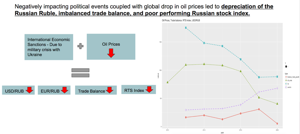
• The oil industry is Russia’s largest industry. In 2012, oil, gas, and petroleum contributed to over 70% of the country’s total export. Russia’s economy was hurt badly when oil  dropped by over 50% in a span of six months in 2014.
• There were international trade sanctions in response to Russia’s military interference with Ukraine’s politics. This had a negative effect on Russia’s economy as there is a rise of instability.

These two factors initiated a “snowball.” negatively impacting the following base economic indicators:  

• The Russian ruble
• The Russian Trading System Index (RTS Index)
• The Russian trade balance

Labels for the chart: Blue - RTS Index, Green - Global Oil Price, Purple - USD/Ruble Exchange Rate,  Red - Russia’s Trade Balance

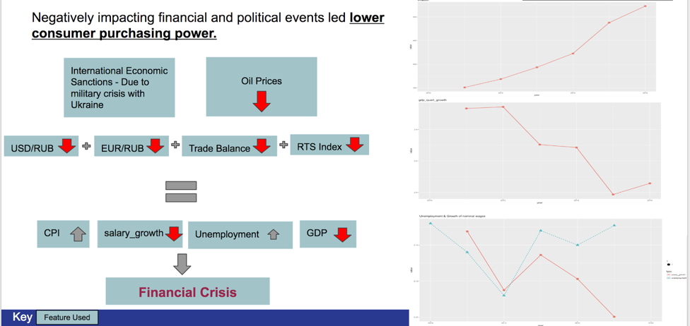
The poorly performing Russian economy manifested a series of changes in Russia’s macroeconomic indicators, including but not limited to:

• Significant increase in Russia’s Consumer Price Index (CPI)
• Worsened salary growth and unemployment rate
• Decline in Gross Domestic Product (GDP)

The change in these indicators, led us to the understanding that Russia is facing a financial crisis.

The first chart measures CPI, the second chart measures GDP growth, and the third chart measures unemployment rate (blue) and salary growth (red)

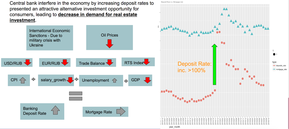
As we continued to explore the macroeconomic dataset, we were able to further confirm Russia’s financial crisis. We observed that the Russian Central Bank had increased the banking deposit rate by over 100% in 2014 in an attempt to bring stability to the Russian economy and the Russian ruble.

In the chart above, the red data points represent banking deposit rates, and the blue data points represent mortgage rates.

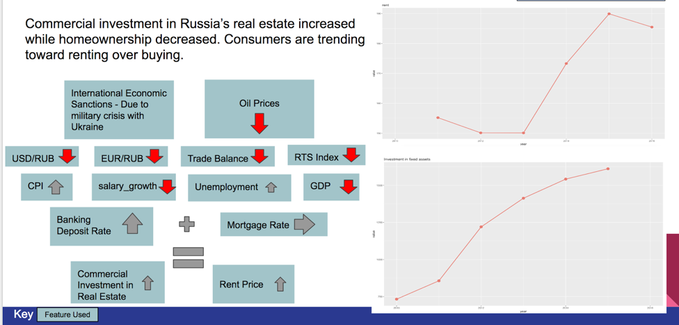
Next, we looked for the effect of the Russian Central Bank’s move on the Russian housing market. When raising banking deposit rates, the Russian Central Bank encouraged consumers to keep their savings in the banks and minimize the public's’ exposure to financial risk. That was seen clearly in the Russian housing market following the raise in deposit rates. We noticed that rent prices increased, and the growth of commercial investment in real estate dropped in the beginning of 2015.

The first chart above represents the index of rent prices, and the second chart shows the level of investment in fixed assets.

This analysis led us to the understanding that the Russian economy was facing a major financial crisis, which significantly impacted the demand in the Russian housing market. This highlights the importance of the usage of the macroeconomic features in our machine learning model to predict the Russian housing market.

The illustration on the left shows the count of transactions by product type. The illustration on the right provides a more detailed view of the same information.

Exploratory Data Analysis

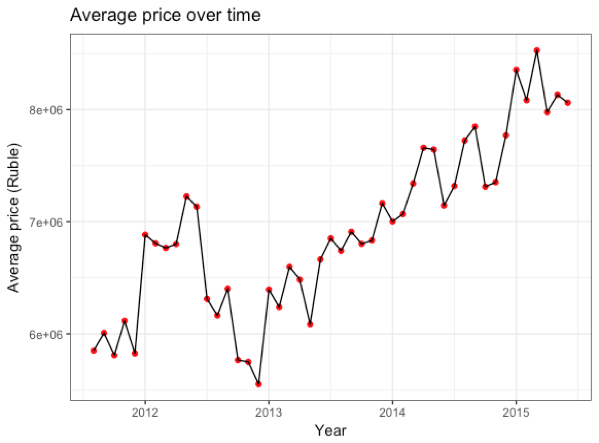
The first step to any data science project is simple exploration and visualization of the data. Since the ultimate purpose of this competition is price prediction, it’s a good idea to visualize price trends over the time span of the training data set. The visualization below shows monthly average realty prices over time. We can see that average prices have seen fluctuations between 2011 and 2015 with an overall increase over time. There is, however, a noticeable drop from June to December of 2012.  

It is important to keep in mind that these averaged prices include apartments of different sizes; therefore, a more “standardized” measure of price would be the price per square meter over the same time span. Below we see that the average price per square meter shows fluctuations as well, though the overall trend is quite different from the previous visualization.

The data set starts off with a decline in average price per square meter, which sees somewhat of an improvement from late 2011 to mid 2012. Again we see a price drop from June to December of 2012.

Some other attributes to take into consideration when evaluating the price of an apartment are the size of the apartment and the size of the building.  

Our intuition tells us that price should be directly related to the size of an apartment, and the the boxplot below shows that the median price does go up relative to apartment size, with the exception of “Large” apartments having a median price slightly lower than apartments of “Medium” size. Factors such as neighborhood might help in explaining this anomaly.

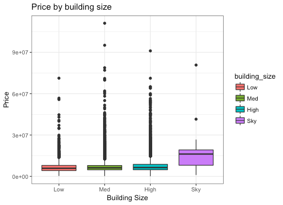
Apartment price as a function of building size shows similar median prices for low-rise, medium, and high-rise buildings. Larger buildings labelled “Sky” with 40 floors or more show a slightly higher median apartment price.

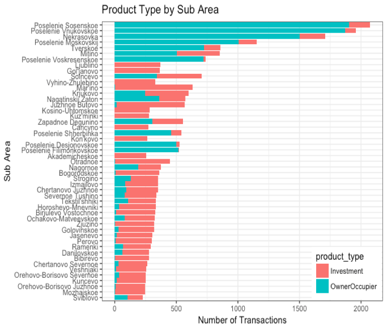
Another interesting variable worth taking a look at is the type of transaction or “product type” mentioned in the data set. This feature of the data categorizes each transaction as being either an Investment or an Owner Occupied purchase. The barplot below gives a breakdown of the transactions for the top sub-areas (by frequency) based on the product type.

This visualization clearly shows that certain areas are heavily owner occupied while other areas are very attractive to investors. If investment leads to increasing prices, this trend will be important for making future predictions.

If we shift our focus to transactions related to the building’s build year based on product type, we see that older buildings generally are involved in investment transactions, possibly due to better deals, while newer constructions are predominantly owner occupied.

Simple exploration and visualization of the data outlines important considerations while training our machine learning model. Our model must consider the factors behind the price dips in 2012 and learn to anticipate similar drops in future predictions. The model must also understand that low prices attract investors, as can be seen with older buildings. However, if investment leads to an increase in price for a particular building, the model must be able to adjust future predictions for that building accordingly. Similarly. the model must be able to predict future prices for a given sub-area that has seen an increase in average price over time as a result of investment.

Feature Selection

To simplify the feature selection process, we fitted an XGBoost model containing all of the housing features (~290 features) and called its feature importance function to determine the most important predictors of realty price. XGBoost was very efficient in doing this; it took less than 10 minutes to fit the model.

In the illustration below, XGBoost sorts each of the housing features by its Fscore, which is a measure of variable importance in its predictive power of the transaction price. Among the top 20 features identified with XGBoost, a Random Forest was used to further rank their importance. The %IncMSE metric was preferred over IncNodePurity as our objective was to identify features that can minimize the mean squared errors of our model (i.e. better predictability).

In order to determine which macroeconomic features were important, we joined the transaction prices in the training set with the macroeconomics by the timestamp and then repeated the process above. The top 45 ranking features are outlined below. In this project, we have used experimented with different subsets of these features to fit our models.

Feature Engineering

Often times it is crucial to generate new variables from existing ones to improve prediction accuracy. Feature engineering can serve the purpose of extrapolating information by splitting variables for model flexibility or dimension reduction by combining variables for model simplicity.

The graphic below shows that by averaging our chosen distance-related features into an average-distance feature, we yield a similar price trend as the original individual features.

For simpler models sub areas were limited to the top 50 most frequent with the rest classified as “other.” The timestamp variable was used to extract date and seasonal information into new variables, such as day, month, year, and season. The apartment size feature mentioned earlier during our exploratory data analysis was actually an engineered featured using the living square meter area of the apartment to determine apartment size. This feature served very valuable during the imputation of missing values for number of rooms in an apartment. Similarly building size was generated using the maximum number of floors in the given building.

Data Cleaning

Among 45 features selected, outliers and missing values were corrected as both the multiple linear regression and gradient boosting models do not accept missing values.

Below is a list of the outlier corrections and missing value imputations.

Outlier Correction

• Sq-related features: Imputed by mean within sub area
• Distance-related features: Imputed by mean within sub area

Missing Value Imputation

• Build Year: Imputed by most common build year in sub area
• Num Room: Imputed by average number of rooms in similarly sized apartments within the sub area
• State: Imputed using the build year and sub area  

Model Selection

Prior to fitting models, it is imperative to understand their strengths and weaknesses.

Outlined below are some of the pros and cons we have identified, as well as the associated libraries used to implement them.

Multiple Linear Regression (R: lm, Python: statsmodel)

• Pros: High Interpretability, simple to implement
• Cons: Does not handle multicollinearity well (especially if we would like to include a high number of features from this dataset)

Gradient Boosting Tree (R: gbm & caret)

• Pros: High predictive accuracy
• Cons: Slow to train, high number of parameters

XGBoost (Python: xgboost)

• Pros: Even higher predictive accuracy, accepts missing values
• Cons: Relatively fast to train compared to GBM, but higher number of hyperparameters

Multiple Linear Regression

Despite knowing that a multiple linear regression model will not work well given the dataset’s complexity and the presence of multicollinearity, we were interested to see its predictive strength.

We began by validating the presence of multicollinearity. In the illustration below, green and red boxes indicate positive and negative correlations between two features. One of the assumptions of a multiple linear regression model is that its features should not be correlated.

Violation of Multicollinearity

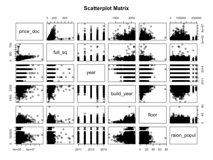
We continue to examine other underlying assumptions of a multiple linear regression model. When examining scatterplots among predictors and the target value (i.e. price), it is apparent that many predictors do not share a linear relationship with the response variable. The following plots are one of many sets of plots examined during the process.

Violation of Linearity

The Residuals vs Fitted plot does not align with the assumption that error terms have the same variance no matter where they appear along the regression line (i.e. red line shows an increasing trend).

Violation of Constant Variance

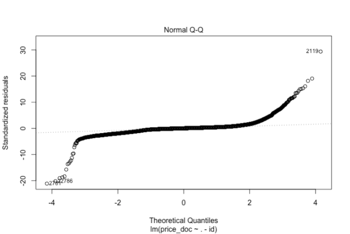
The Normal Q-Q plot shows severe violation of normality (i.e. standardized residuals are highly deviant from the normal line).

Violation of Normality

The Scale-Location plot shows a violation of independent errors as it is observed that the standardized residuals are increasing along with increases in input variables

Violation of Independent Errors

Despite observing violations of the underlying assumptions of multiple linear regression models, we proceeded with submitting our predictions to see how well we can score.

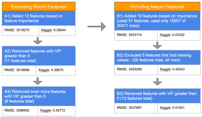
Our first model A1 was trained using the top 12 property-specific features identified in the feature selection process. Submitting predictions using this model gave us a Kaggle score of 0.39544 on the public leaderboard (this score is calculated based on the Root Mean Squared Logarithmic Error). Essentially, the lower the score, the more accurate the model’s predictions are. Nevertheless, it is possible to “overfit the public leaderboard”, as the score on the public leaderboard is only representative of the predictions of approximately 35% of the test set.

Models A2 and A3 were fitted by removing features from model A1 that showed VIFs (Variance Inflation Factors) greater than 5. Generally, features with VIFs greater than 5 indicate that there is multicollinearity present among the features used in the model. Removing these did not help to improve our Kaggle scores, as it is likely that we have removed features that are also important to the prediction of price.

Models B1, B2, and B3 were trained with the features in A1 with the addition of identified important macro features. These models did not improve our Kaggle scores, likely for reasons mentioned previously.

Gradient Boosting Model

The second machine learning method we used was the Gradient Boosting Model (GBM), which is a tree-based machine learning method that is robust in handling multicollinearity. This is important as we believe that many features provided in the dataset are significant predictors of price.

GBMs are trained using the bootstrapping method; each tree is generated using information from previous trees. To avoid overfitting the model to the training dataset, we used cross-validation with Caret package in R. Knowing that this model can handle complexity and multicollinearity well, we added more features for the first model we fitted.

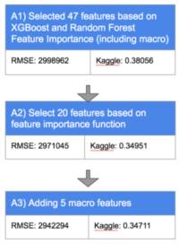
In Model A1, we chose 47 features from the original training dataset, which gave us a Kaggle score of 0.38056. Next, we wanted to check if reducing the complexity of the model gives better results. We decided to run another model (A2) with only 20 features. This model performed better than Model A1.

In Model A3, we added to the previous model, 5 macro features that were chosen using XGBoost feature importance. As expected, the macro features improved our results. The model gave us the best Kaggle score of all the gradient boosting models we trained.

For each of the GBM models, we used cross-validation to tune the parameters (with R’s Caret package). GBM models on average provided us better prediction results compared with those using the multiple linear regression models.

XGBoost

An extreme form of gradient boosting, XGBoost, is the preferred tool for Kaggle competitions due to it’s accuracy of predictions and speed. The quick speed in training a model is a result of allowing residuals to “roll-over” into the next tree. Careful selection of hyperparameters such as learning rate and max-depth, gave us our best Kaggle prediction score. Fine tuning of the hyperparameters can be achieved through extensive cross-validation; however, caution is recommended when fitting too many parameters as it can be computationally expensive and time consuming. Below is an example of a simple grid search cross validation.

Prediction Scores

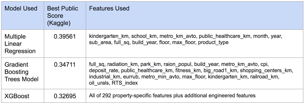
The table below outlines the best public scores we have received using each of the different models, along with the features used.

Future Directions

This two-week exercise provided us the opportunity to experience first-hand what it is like to be working in a team of data scientists. If given the luxury of additional time, we would dedicate more to engineering new features to improve our model predictions. This would require us to develop deeper industry knowledge of Russia’s housing economy.

Acknowledgement

We thank the entire team of instructors at NYC Data Science Academy for their guidance during this two-week project and also our fellow Kagglers who published kernels with their useful insights.