Housing Prices Prediction using Machine Learning
The skills I demoed here can be learned through taking Data Science with Machine Learning bootcamp with NYC Data Science Academy.
Project Overview
Objectives
What makes a house a good buy? Which particular aspects of your house or the house that you’re looking to buy can make it more or less expensive, given all other things stay intact? When is the best season to sell, or best season to buy? How much less will your house cost if you wait another year to sell it? Is having a large basement makes a house more attractive to potential buyers?
The Data
Data itself was obtained from the Kaggle website, particularly from the House Prices: Advanced Regression Techniques competition. The dataset contains 79 variables that describe almost every possible aspect of a residential property. Features range from the size of the property to its geographical positioning relative to city facilities, from the presence of the additional amenities to their overall quality, from the materials used to build the roof to the year when the house was last renovated
Data Preprocessing
Missingness and Imputation
Like any data collected from in the ‘real world’, some of the variables in the dataset had a fair share of missing values. However, not all missingness is created equal. Therefore each of the variables required a closer examination.
First type of missingness, which we called “fully explained missingness”, is mainly connected to the presence or absence of certain amenities. For instance, if the house does not have a garage, it has an “NA” in the column “Garage Type”. This means that the house simply does not have a garage, and data is not actually missing. Therefore, such NA values have been substituted with “No Feature” variables.
Another type of missingness is entirely derived from the previous one. In other words, the value in the particular column was missing or for numeric values was equal to zero solely based on the values of another column. Continuing with the Garage example, if the house had no Garage, therefore has a zero in the column “Garage Area” or “Garage Year Built”. Thus, it didn’t require additional imputation.
Third type of missingness is what is called “Missingness Completely at Random”, which means that several values in some of the columns seem to be missing without any evident pattern and any connection to other features. Their missingness can best be explained by mistake during data collection. In this case, our team used ‘median’ imputation for numeric variables, and ‘majority vote’ imputation for categorical variables.
Outliers
One of the most important parts of the data preprocessing is the removal of outliers. Outliers, even when their amount is insignificant, can noticeably skew the model, and, especially for linear models. That’s why their examination and subsequent removal or transformation is often crucial.
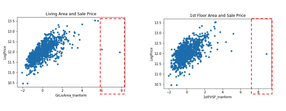
By plotting the relationship between independent variables vs. the price, we were able to observe the outliers mentioned above.
Some of the outliers were observed in variables such as the Living Room area and First Floor Area.
Another type of outliers occurred in categorical variables (both nominal and ordinal) and could be mostly explained by category having a very small number of homes in it.
Insignificant Features
Sometimes, even after taking into account all the types of missingness and performing all the appropriate imputations, variables still contain such an enormous amount of missing values, that using them will not only not contribute to a better model, but will only make it less accurate in predicting the actual values.
One of the examples of such features is the Pool Area and Pool Quality. Both of which are missing 99.65% of all the values. They have virtually no variance, and cannot add any information to our future model. Therefore, these kinds of variables were dropped.
Another example of insignificant features includes LowQualitySF, where 98% of values are zeros, or Heating Type, where 98% of the values belong to one category.
New Features Creation
Some of the features, while being useful overall, are not presented in the form best suitable to perform model building. Also, some of the features are too sparse, which makes them have significant missingness on their own, but when combined, they can give us a much better picture and can significantly aid the analysis.
Some of the features created from the manipulation of other features included:
Age = Year Sold - Year BuiltTotal porch = Open Porch + Enclosed Porch + Screen Porch + 3Ssn Porch
Garage Age = Year Sold - Year Built
Data Transformation
Before data can be “fed” into the model, we need to examine it for normality, and then try to transform it if it is skewed, or not normally distributed. Some of the transformations applied to our features included log transformation, square root transformation, as well as squared log transformations.
For example, the log transformation has been applied to a newly created Total Porch variable in order to remedy its skewness of the data.
For the purposes of analysis, the dependent variable (House Price) has also been log-transformed to ensure greater normality and linearity.
Preliminary Assumptions
First, before starting model building, it is crucial to take a general look at the data. What are some of the assumptions that we can make about features’ influence on the housing price before we go on with creating a model? Is there any apparent linearity that can give us a hint on how this feature makes the price go up or down?
We can observe a degree of correlation between some of the variables and the final house price. Many of the variables seem to confirm our intuition. For example, the older the house, the lower on average its price appears to be. Another great linearity example is the “Overall Quality” variable, whose correlation with the price seems to follow our reasonable assumption. The higher the quality of the house, the higher the price of the house.
Standardization and Encoding
The final step before training the model is to standardize some variables and encode the others.
Ordinal variables, such as the ones that demonstrate the quality, for example, were transformed into numeric variables, as they have a definite order in their structure. (e.g., “excellent” is clearly greater than “good”).
Numerical and ordinal variables have been standardized using the sklearn StandardScaler, which subtracts the mean and then transforms all variables to unit variance. The mean of the standardized collection of observations is equal to zero, and observations follow a standard normal distribution.
For the categorical values, the OneHotEncoder was used to encode values and prepare them for model tuning.
Machine Learning
Model Performance
For predictions, the team has built, tuned, and trained four models. The models are Ridge, Lasso, Gradient Boosting, and Ensemble model, which included all three models mentioned prior. The best Kaggle score that the team was able to achieve is 0.12163, which is the Root Mean Squared Error (RMSE) between the logarithm of the predicted value and the logarithm of the observed sales price. The model that gave the best result is the Ridge Penalized Regression. Other models provided us with some other decent scores.
Key Findings
Arguably, an even more important part than the model accuracy is the model interpretation. In other words, by looking at variables and coefficients, how appropriately and comprehensively can we explain the importance of a particular variable, and how can we measure its importance.
Building several models, with different accuracy, allowed us to examine differences in “feature importance”, and compare which variables seem to stay important between models. While some of the models give us slightly less accurate predictions, they can tell us more about which aspects of the residential property are more important.
Model Interpretation
After the model is ready, it is time to find out what the coefficients actually mean. Since we transformed, merged, and standardized our features, it is now crucial to convert the coefficients back into the more “direct” numeric form.
The table below demonstrates some of the examples of how coefficients can be transformed into the “price percentage increase”.
Feature importance
The picture below demonstrates the importance of features according to the two most interpretable models.
We can observe that features like the Size of the Living Area, Age of the House, and Overall Quality stay very significant across the models.
Some of the most important features have been grouped into four categories, presented in the picture below. Key variable groups are Location, Size(sq. footage), Presentability, Time & Circumstance.
Recommendations
Ways to add value
Finally, we want to see what are the actual, straightforward suggestions that the model can give us regarding the changes that can be made to the house, in order to increase its values or suggestions that can help us to choose the time to buy a home when prices are generally lower.
One of the variables we can take a look at is the Month of the Sale. The base month, to which we are going to compare price variations, is June. The worst month to sell a house is October, since prices in October tend to be, on average, 3% lower than the price for the exact house in June. On the other hand, the best time to sell, and hence probably the worst time to buy is May, owing to the fact that the average price of the house in May tends to be more than 2% higher than in June.
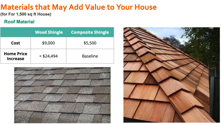
Another variable that has a direct influence on the price of the house, and is the feature that the house owner can actually control is the “Roof Material”. Changing the material with which the roof was built can directly increase the average sale price of the house.
In our case, we can compare the price of different roof option installation, to the most common roof material, which is Composite Shingle. The average price of the installation of Composite Shingle Roof for the 1500 sq.ft size house will is - $5,500. At the same time, the installation of the Wood Shingle roof, for the house of the same size, will cost, on average, $9,000, but at the same time, it will increase the average sale price by almost $25,000. We conclude that changing the roof material is, in most cases, absolutely worth it.
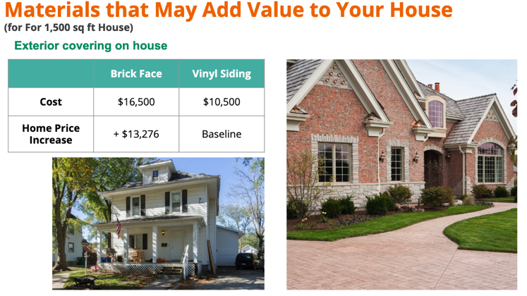
Another example of a useful exterior modification is Exterior Covering material. According to the model, changing your house covering can increase the final price of your house, with other things equally considered. Most noticeably, covering your house in Brick Face, can increase the price of the house by more than $13,000. While installing the brick face costs only $6,500 more than the most common exterior covering - Vinyl Sliding.
Conclusions
In general, the models built, allow us to both make reasonably confident predictions of the actual prices, and understand the importance and the role of the features crucial in making the predictions.
In many ways, the outcome has proven right many of our intuitive assumptions regarding what determines the value of the house. Features like Overall Quality, Total Living Area, and Age are expected to have the strongest influence on the price of the house. On top of the other features directly or indirectly connected to the area, such as Lot Area, Garage and Basement Area. Finally, as it is often said, “Location, Location, Location”, often plays an important role. Neighborhood in which the house is located, as well as its proximity to various amenities or disturbances, have a significant influence on the final house price.
Thank You
Thank you for taking the time to read our blog. You can follow the link to the GitHub if you’re interested in learning more about the process behind the analysis.
The Team
The group “Tea-Mates” consists of Ting Yan, Marina Ma, Alex (Oleksii) Khomov, Lanqing Yang.


