What We Learnt From Higgs Boson Challenge

EDA

The project focuses on the detection of the Higgs boson signals in a particular CERN ATLAS accelerator simulated data. The data set consists of two portions. The train set consists of 250K observations, with two-class labels on the signal (about 1/3) and the background (about 2/3), and the data weights which underweight the signals to reflect the rareness of the Higgs signal in reality. The test set consists of 550K unlabeled observations. The goal is to apply machine learning classification algorithms to separate the signal from the background, with the performance gauged by a specific approximated median significance (AMS) score designed by the particle physicists.

Among the thirty variables of both the train/test data sets, there are eleven variables with missing values, several of them miss up to 2/3 of the observations. This poses a particular challenge to impute the missing data, in order to be processed by the machine learning algorithms.

It turns out that the appearance of missing values is controlled by one categorical variable jet_num (with the values 0, 1, 2, 3), except the missing values of the predicted Higgs mass.

The term 'jet' is used to describe that in the high energy proton-proton collision, the near light-speed proton particle pairs get shattered into many fragments, consisting of the decay products of quarks, gluons emitting like shotgun showers focused in some particular direction in space. In the experiment of the Higgs boson discovery, there can be either no jet, one jet, two jets, or three jets or more in a single proton-proton collision. The physics involving the different number of jets can be significantly different, which result in different probabilities of the signal candidate events.

The probability of finding Higgs signal candidate varies with respect to the number of jets

We first summarize the pattern of missing values by the following hierarchical clustering Dendrogram,

The hierarchical clustering analysis on the boolean matrix of whether the entry has missing values

In the above dendrogram plot, the leftmost single cluster MASS_MMC is the predicted Higgs mass.
It has the unique missingness pattern different from the pattern of the missing values of the other variables. The second cluster consists of 19 variables with no missingness at all. On the right, there are two clusters of seven and three elements, respectively. The seven-element cluster collects the variables describing the double-jet physics. They become missing when the num_jet drops below 2.
The rightmost three element cluster describes the physics of the leading jet (the one with the highest energy if there are more than one jet involved). They become missing exactly when the num_jet is equal to zero.

Even though the categorical variable num_jets do not explain the variations of the Higgs signal rates at different scattering angles, it controls the behavior of the underlying particle physics. Its importance cannot be ignored. The tree type machine learning can handle continuous as well as categorical variables well. It will be the focus of our discussion.

We point out that the predicted Higgs mass MASS_MMC is missing when the formula deriving the mass from the other primary measured quantities does not produce the physically meaningful Higgs masses. When this situation occurs, the chance of the appearance of Higgs signals is greatly reduced. This is manifest in the following table,

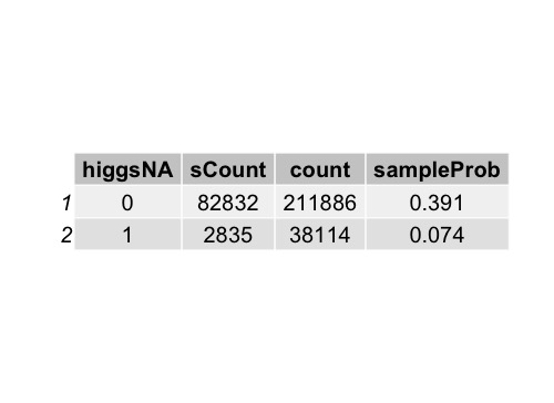
When the predicted Higgs
mass is missing, the probability of getting signal drops to 7% from nearly 40% (when the predicted mass is not missing).

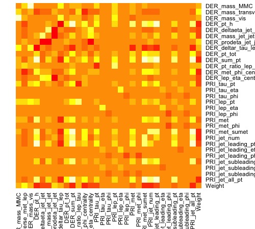
We observe that the 30 variables often display high linear correlations,

The correlation among the 30 variables. Red is negative correlation, yellow is positive correlation

Among the thirty variables, there are primary raw variables as well as the derived variables. The derived variables are often nonlinear functions of several primary raw variables, attempt to capture
nonlinear relationships between the raw variables. So it is not surprised that they are correlated with each other. Among the primary (raw) variables, there are also nontrivial correlations. It often makes training the machine learning algorithm challenging.

Due to the special nature of the missingness, the scheme of 'missing at random' (MAR) imputation is not ideal. They often make the missing values mimicking the variable's population distribution. In our situation, the values' being missing are NOT because the values exist but do not show up in the record. They are missing simply they do not exist in the particular scenario. Imputing the missing value by mean/median or other sophisticated methods without checking the basic imputation assumption ruins the internal meaning of the data (along with energy conservation ....) and introduces unpredictable noises to the machine learning algorithms downstream.

Logistic Regression

As discussed through EDA, linear classification models were not expected to perform well on this dataset. However, logistic regression was still picked as the first model to be tested. There are several reasons to use this model:

1. It only takes a few seconds to train a logistic regression model and make predictions on testing data. This allows users to start working on later steps of the project, including selecting prediction threshold, and transforming predictions into the proper format that can be submitted to Kaggle for evaluation.
2. Logistic regression can be easily interpreted. This helps users to further understand how independent variables affects the outcome of each observation.
3. Logistic regression provides a good performance benchmark. While advanced models tend to give more accurate predictions,  the algorithms generally become more complicated and hard to interpret. To decide whether the predictive power of a "black box" model is good enough to overcome its lack of interpretability, users can compare the model's performance with the performance of logistic regression to make their judgment calls.

Without any data imputation, a simple logistic regression built on all variables reached a 0.816 AUC score, and the test set AMS is 2.02.

ROC curve of Logistic Regression Model

Summary of Logistic Regression Model

Random Forests

The random forest is an ensemble of tree models, which overcomes the drawbacks of the single tree model
and often offers high accuracy comparable with the other advanced supervised machine learning algorithms. When we tested on the train set using the random forest algorithms, we noticed early on that the optimal model after 10-fold cross validation produces a peculiar almost perfect in-sample AUC.

The mtry=3 optimal Random Forest in-sample fit after 10-fold cross-validation training. It looks like 'overfitting'

Is it an 'over-fitting' model? Let us review its variable importance plot,

The top of the variable importance plot indicates that the predicted Higgs mass is most important!

The top three important variables, according to this optimal random forest, are all mass-related.
They are predicted Higgs mass (MASS_MMC), the transversal invariant mass between the lepton (electron or muon) and the undetectable neutrino, the invariant mass between the lepton and the hadronic tau.

In the EDA section, we have noticed the predicted Higgs mass as the strong indicator of the presence of the signal events. So it becomes puzzling and intriguing at the same time that if the model is indeed over-fitting (misidentifying the noises as some patterns), how could it pinpoints a strong predictor and puts it on the top of the variable importance list? If it is not overfitting, why does the test AMS score is below 3.0, not even ranking among the top 1000?

In the rest of the section, we will do the detective work and offer the reader a rational explanation for this phenomenon and the way to fix it.

We borrow the idea of the binary search and separate the variables into the complete and non-complete (with missingness) groups. It turns out that the AUC is still 1 for the 19 variables optimal RF! Thus we know that this phenomenon is independent to the imputation of the missing values. Moreover, the lepton-neutrino transversal invariant mass and the lepton-hadronic tau invariant mass are on the top of the list (predicted Higgs mass has missing values, so it is absent from the complete variables group), with fast falling mean Gini Index. This motivates us to drop all the other variables except these two. Again we see the same AUC=1! Now the situation is simple enough for us to provide a detailed analysis.

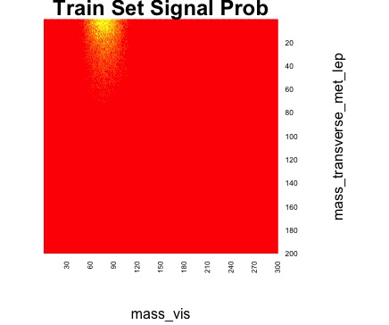
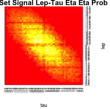
In the following, we consider the probability heat maps of the events falling onto the lepton-neutrino transverse invariant mass vs lepton-tau invariant mass plane. 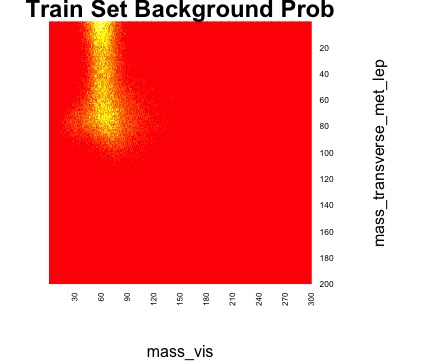 The background events fall onto the upper left of the rectangular heat map. The red is near zero. The yellow is the locations where the events accumulate.[/caption]

The signal events fall onto a much more concentrated region on the upper-left of the heat map.

It turns out that the different patterns of the signal-background can be discerned by the human naked eyes, let alone by the sophisticated ML algorithms. To show that these pattern distinctions are not isolated, we display two other pairs of variable heat maps.

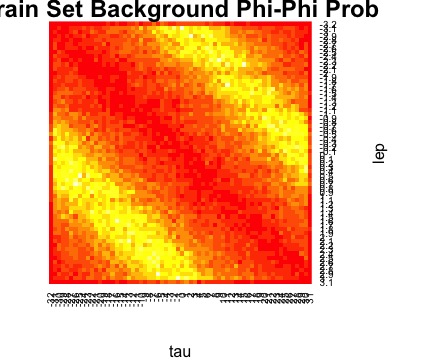
The first one is lepton Phi angle vs tau Phi angle heat maps,

The background events lepton vs tau scattering angles heat map

The signal events lepton vs tau scattering angles heat map

We observe the apparent distinct patterns on the scattering angles [Latex]\Phi[/Latex]. For the Higgs-like proton-proton scattering, the sum of the lepton and hadronic tau scattering angles is either 180 degrees or -180 degrees. The restriction on the background events is much weaker.

The background events lepton vs tau pseudo-rapidity heat map

The signal events lepton tau pseudo-rapidity heat map

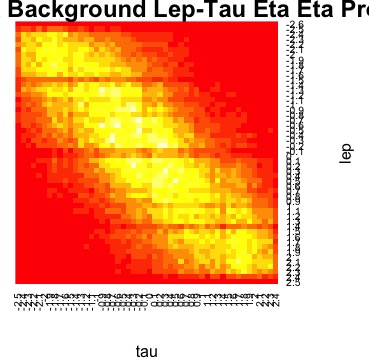
The pseudo-rapidity parametrizes the scattering angle with respect to the incoming proton beam. The signal events and the background events have different heat map patterns.

These examples illustrate that among the 19 complete variables (with no missingness), there are a lot of apparent patterns which the random forests or other machine learning algorithms can identify. If the random forests do help us to identify the strong pattern, why does it fail to perform as well on the test set?

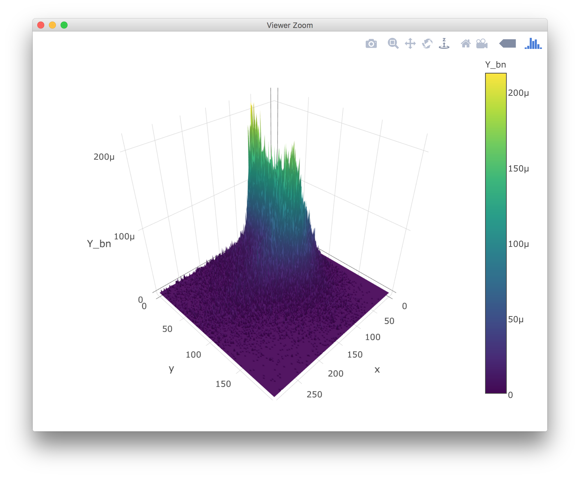
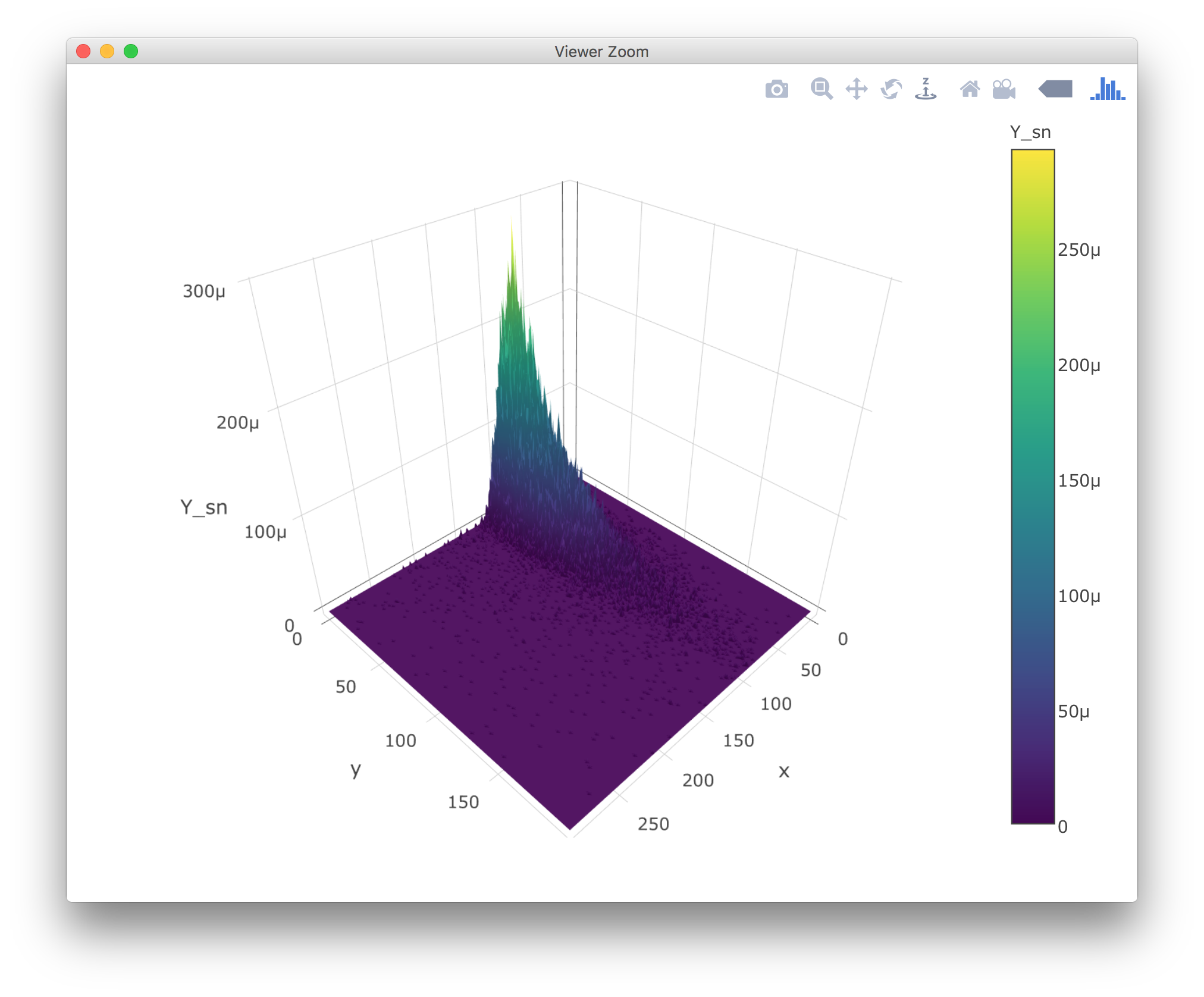
To reveal this, we plot the probability densities in terms of 3D plots,

The background events probability density 3D plot

The signal events probability density 3D plot

The random forests technique learns about the pattern by estimating the probability density functions using piecewise constant functions, cutting the domain into many small rectangular shaped blocks. it is a big advantage that the random forests do not make any assumption on the function form. But when the shape of the out of sample probability density functions shift, the original piecewise constant approximation of the original probability density function could be a poor approximation to the test sample probability density function. To understand this, we display the 3D plot of the difference of the test-train total (signal+background) probability density functions,

The gap between the test and train samples signal probability distribution plots

Given the 1 GEV unit of the grid, the scale of the probabilities is in [Latex]10^{-6}[/Latex]. We notice that the difference of the test set (signal and background combined) distribution from the train set distribution can go as high as [Latex]90\times 10^{-6}[/Latex], about one-third of the maximal values of the distribution itself. Such a big fluctuation on the sample probability distributions can throw the estimates of the class (signal or background) probabilities off. After the 10-fold cross-validation training, the optimal 2-variable model can predict almost perfect accuracy, making only three errors. But such an intimate knowledge of the signal/background distribution does not generalize well if the probability distribution varies significantly.

To resolve the 'overfitting' issue, we need an effective way to prevent the random forests to look into an extremely high resolution which does not generalize well in the high noise condition. An excellent candidate is to increase the 'nodeNumber' from the default value 1 to the higher values. Empirically, we find that if we change the nodeNum from 1 to 100 or above, we can effectively reduce the overfitting on the train set but still keep the same AMS score on the test set. This demonstrates the root of the problem comes from a miscalibrated random forest learning algorithm from the R package to deal with the extremely noisy situation.

The 250K training and 550K test data seem like large, but in the content of the accelerator physics, it takes about 1 second to generate 200K events. So there is no wonder that the roughly 1 second worth of training set and the 2+ seconds worth of test data can show a significant difference in their sample probability distributions. After all, one needs to scan through the time series data to estimate the hidden population density distribution.

eXtreme Gradient Boosting (XGBoost)

Although random forest has been proven not working well on this dataset, there are many other tree models can be tested. Boosted tree model, for example, is another well-recognized tree model that usually give outstanding performances on classification problems. XGBoost, as one of the advanced implementations of boosted tree algorithm, is famous for its fast speed, high accuracy, and most importantly, capable of handling special encoding for missing data (-999 in this case). Therefore, XGBoost was tested as the last algorithm to build the predictive model on this Higgs Boson detection dataset.

One problem of using XGBoost model is hyper-parameter tuning. The author of XGBoost has made the tool extremely flexible, which allows users to customize a wide range of hyper-parameters while training the model. Therefore, to reach the optimal solution, users need to try massive amount of different combinations of hyper-parameters. While this flexibility allows users to push the limit of this tool, it also makes the parameter-tunning process extremely time-consuming and sometimes relies on luckiness. Since it is visibly impossible to try all possible parameter combinations, we only focused on several important parameters that make major impacts on model performance. For example, depth of each tree, the number of variables and observations that can be used while building each decision tree, and evaluation metric. To be more efficient on parameter searching, we firstly used a two-fold cross-validation to fastly scan through a wide range of parameter values, narrow down the search range based on validation set AMS and AUC scores of each combination, and then apply a five-fold cross-validation to further scan for the optimal parameters.

The final model was trained with max depth = 6, learning rate = .1, and 90% of observations as well as variables were used when constructing each decision tree. As the result, the final model scored 3.5 AMS on Kaggle's test set. The feature importances of this final model is very similar to the ones of random forest, but performing much better on predicting testing set signals, which suggests that boosted tree model is less sensitive to the signal pattern shifts between the training and testing sets.

Feature Importances of XGBoost Model

The Codes

For the observation on the importance of the num_jets and the predicted Higgs mass, we have Higgs mass/num_Jets affect probability of the signal appearance

For the Higgs data imputation, we have HiggsDataImputation

For the data preprocessing and the random forest algorithm training random forest

For the analysis using hierarchical clustering, we have hierarchical clustering of the features

For the 3D plots using plot_ly and the data conversion, we have process data into the sample probability density

For the heat maps using the base R heat map, we have heatMaps of the patterns