Machine Learning Techniques for Predicting House Prices
By Weijie Deng, Han Wang, Chima Okwuoha, and Shiva Panicker
For decades the American Dream has been defined by the pursuit of home ownership, and in 2017 Zillow reported that the median value of U.S. homes hit a record high of $200,000. Housing prices are determined by a slew of factors; some quantifiable, and some not. Being able to isolate the best factors for predicting housing prices has a clear use for real-estate investors as well as individuals looking to move into a new home. In this project, we used, compared, and stacked multiple machine learning algorithms to predict housing prices in Ames, Iowa.
Dataset/ Data Cleaning
The data set included 80 variables, each that have a varying impact on the final housing price. The variables included details about the lot/land, location, age, basement, roof, garage, kitchen, room/bathroom, utilities, appearance, and external features (e.g., pools, porches, etc.).
The data frame provided was relatively clean, which allowed us to focus on making the variables compatible with our models.
After looking at the Sale Price feature, we saw that it did not follow a normal distribution, so we decided to transform it to better represent a normal distribution. The transformation we used was a logarithmic transformation of the form log(price + 1).
After transforming the sale price, we noticed several numeric features were not normally distributed. This was problematic, as certain linear models are based on the assumption that predictors are normally distributed, and violating these assumptions could negatively affect the linear model, thus making predictions inaccurate. To fix this, we decided to skew those with degrees of skewness larger than 0.75.
We filtered the following features to be skewed, which were '1stFlrSF', '2ndFlrSF', '3SsnPorch', 'BsmtFinSF1', 'BsmtFinSF2', 'BsmtHalfBath', 'BsmtUnfSF', 'EnclosedPorch', 'GrLivArea', ‘'KitchenAbvGr', 'LotArea', 'LotFrontage', 'LowQualFinSF', 'MasVnrArea', 'MiscVal', 'OpenPorchSF', 'PoolArea', 'ScreenPorch', 'TotRmsAbvGrd', 'TotalBsmtSF', 'WoodDeckSF'. We use the same logarithmic transformation, log(x + 1), to make the features normally distributed.
Now we had to figure out a way to deal with the ordinal features and categorical features.
For the ordinal features, we read in the descriptive text to extract those features, so that we could turn them into numeric features. We fed them into a dictionary and applied them to columns.
For categorical features, we had tried both one-hot encoding and label encoding. In linear models and random forest, dummification had better performance than label encoding. So we use one-hot encoding to handle all the categorical features. One-hot encoding will turn all the items in one predictor into a new column, in which 1 means True and 0 means False, and delete one item to make it obey the linear model assumption.
The graph below shows the features that have a strong linear correlation to each other. Linear features follow the line of best fit such as in the case of case of overall quality predicting sale price. For those colored in red, we can delete one of those two having high correlations. Through this graph, we can easily tell which features have the highest correlation with each other.
3.Models
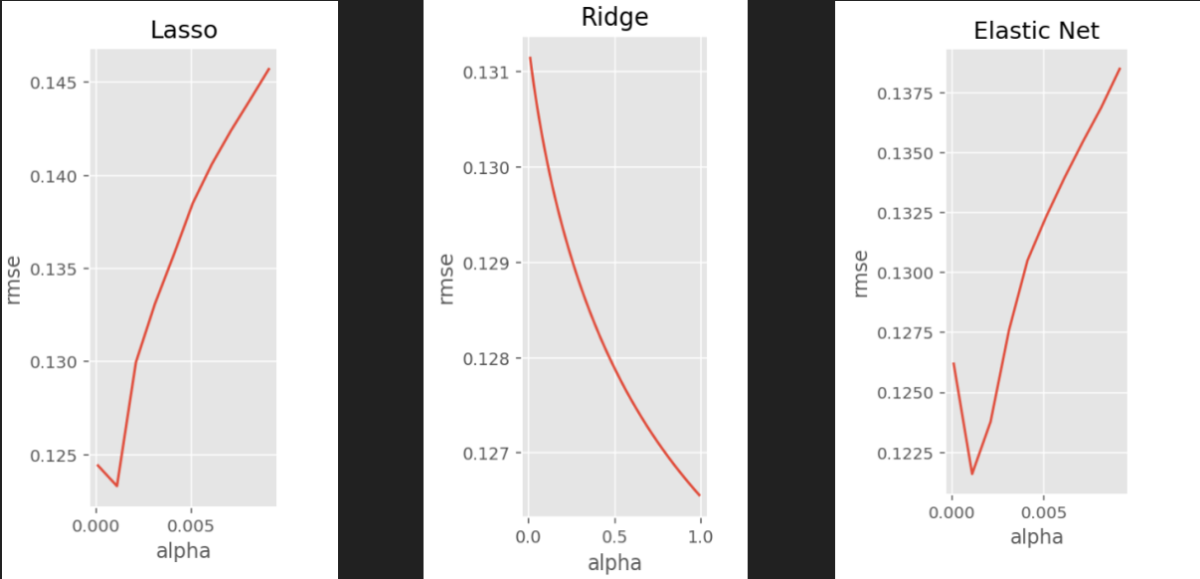
3.1 Lasso, Ridge and Elastic Net
3.2 Gradient Boosting
We used cross validation to find the best parameters for a gradient boosting regression. These parameters were learning_rate = 0.04, max_features='sqrt',n_estimators=500, max_depth=4,subsample=0.7,min_samples_split = 10,min_samples_leaf =2.
The following graph is of the top 30 variable importance. The top two most important variables are "Fence" and "Full Bathroom." However, there is a limitation that when using dummified data to fit tree models-- they will usually be misleading and have incorrect answers.
Although the RMSE of gradient boosting is 0.118, the RMSE on Kaggle is 0.166. This model has a very serious overfitting problem. We considered the problem should result from the tree model.
3.3 Support Vector Regression
The decision to implement a support vector regression was based on the fact that our data was very sparse and was of high dimensionality. Support vector regressions actually perform well in high dimensional scenarios, mainly because in higher dimensions it's easier to construct a hyperplane which splits the data nicely.
To implement the SVR, we used a built-in SVR function in the sklearn module (from sklearn.svm import SVR). SVR is a computationally demanding model, with non-linear kernels being more demanding than the linear kernel, so in the interest of time, we chose to go with the linear kernel for our support vector regression. We set our epsilon to be 0.1 and applied a grid search cross-validation to select the best performing model.
To our surprise, SVR had the lowest performing test score out of all the models, with an RMSE of 0.14602. At first we thought this was due to a poor choice of kernel and epsilon--we thought a non-linear kernel would perform better than the linear kernel we chose to go with. Ultimately though, the low score was mainly attributed to size of our training set. While support vector regressions perform well on high dimensional data sets, they also require a large number of samples to train on. With our data being very sparse after encoding, and having a dimension of approximately 1500x250, the support vector regression did not perform as well as the other models we used.
4.Stacking
| Model | Test Score | Kaggle Score |
| Lasso | 0.122625 | 0.12249 |
| Ridge | 0.128345 | n/a |
| ElasticNet | 0.12554 | n/a |
| Spline | 0.11357 | n/a |
| Random Forest | 0.136219 | n/a |
| SVR | 0.14602 | n/a |
| Gradient Boosting | 0.11896 | 0.16694 |
| Stacking | n/a | 0.16356 |
5. Lessons Learned
a. Data cleaning is arguably the most important and most time consuming task
b. Give a hypothesis of which simple model may work best on the given data
c. Implement the simple model
d. UNDERSTAND the model, and why it gave the output it did
e. Update hypothesis and repeat (2)


