Predicting House Flipping Profits Using ML
According to CNBC, home flipping profits are dropping at the fastest pace in over a decade. If you are in the flipping or renovating business, how do you get the most return for your investment in a volatile housing market? This is what our project set out to do. We used machine learning methods to predict which areas of a house could provide the most value. Of course, each renovation scenario needs to take into account the costs associated, but if we can target areas of the house with high potential return on investment, this would be a valuable starting point for cost-benefit analysis of a flip.
Data
This project uses the Sale Price of Houses in Ames, Iowa, provided by Kaggle. The dataset contains 79 features which describe various aspects of residential homes that were sold in Ames, Iowa. The goal of our modeling was to predict sales price from the other features of the home, so sales price was used as the independent variable. Sales price is a continuous variable which indicates that we need to use a regression model, but which regression model to use took additional analysis. To determine which model to use, we used the following process for our project:
- Clean and pre-process the data
- Conduct Exploratory Data Analysis (EDA)
- Engineer features to capture ‘real-world’ attributes
- Create initial models for exploration
- Select a model type
- Analyze features using various methods
- Create final model using ensemble techniques
- Assess feature contributions to Sales Price
Feature Engineering
After the data was analyzed, we understood that we had many features to work with, but several features could be combined and summarized in two or less features. The following were created using existing features:
- TimeSinceLastWork: Numerical variable that summarizes the last time the house was renovated.
- TotalSF: Numerical variable that was not included in the original dataset, but was captured using the total basement square footage and ground level square footage.
- FinBsmt: Boolean variable that describes if the house has a finished basement or not.
- TotalBathrooms: Numerical variable that captures bathrooms located in the basement and ground levels including half baths.
- OutdoorLiving: Boolean variable that captures outdoor living areas including wood decks, open porches, enclosed porches, three-season porches and screened-in porches.
- HasPool: Boolean variable that captures if the house has a pool or not.
- Fireplace: Boolean variable indicating if the house has a fireplace or not.
Associated variables that were used to create the new engineered features were dropped from the dataset to prevent multicollinearity and redundancy.
Feature Exploration
To understand which features should be included or dropped and their relative importance before modeling, we used the following methods on the non-engineered feature set for exploration:
- Random Feature Subset Analysis: To get a baseline performance, we used 10 randomly selected features to train and test using a Random Forest Model. This returned the highest R² of 78% with the following features:
- GarageQual
- EnclosedPorch
- BsmtExposure
- HalfBath
- YearRemodAdd
- FireplaceQu
- TotalBsmtSF
- GrLivArea
- ExteriorSF
- Fireplaces
- MasVnrArea
- Electrical
- OverallCond
- TotRmsAbvGrd
- SciKit-Learn’s VarianceThreshold(): This function allows you to discover features that have the least amount of variance in your feature set. If the feature has low variance, this feature may not help us identify an increase in SalesPrice.
- SciKit-Learn’s KChooseBest: This function allows for univariate feature selection with the F test. If the feature has a high F value and a low p-value, that may be an indicator that feature will have a statistically significant effect on SalesPrice.
- SciKit-Learn’s SequentialFeatureSelector: This method selects features using a backward selection method. A Random Forest estimator model was used to choose the best features to add or remove based on the highest R²
In summary, features that these methods inferred to leave out were around Utilities, LandContour, MoSold, YrSold, SaleType and other variables containing condition/qualitative properties. Although these feature exploration methods were helpful in feature selection, ultimately we chose to keep all features due to the nature of the model that was selected.
Modeling
We experimented with both Multiple Linear Regression and Random Forest Regression. Based on correlation and VIF (Variance Inflation Factor) values, it was determined that a large amount of multicollinearity, both linear and nonlinear, existed amongst the features. It was not possible to reduce VIF values sufficiently through feature selection. Since Multiple Linear Regression cannot be performed on data with multicollinearity, we chose to move forward with Random Forest. Random Forest can handle correlation and non-linear relationships between features, can produce interpretable results, and is a strong performer.
Random Forest
Using our engineered dataset, we built a Random Forest model and performed hyperparameter tuning using cross validation to maximize the model’s performance. Below is a plot of the 30 most important features determined by the model. The importances are calculated as the Gini importances, or the total reduction of squared error brought by that feature. This model resulted in an R² value of 82.8%.

We then performed a greedy procedure guided by the feature importances determined by the model (figure above) to select only a subset of the features to be used in the final model. This process involved first training the model with only the most important feature and calculating the R² of that model. We then added features, one at a time, in order of importance, and calculated the R² at each iteration. The figure below displays the result of the greedy procedure. The model performance tapered at about 90%, starting when the model was trained with just the top 13 most important features. We therefore decided to build our final Random Forest model using only those 13 features.

The model was trained on the top 13 features and hyperparameter tuning was performed with Random Search CV. This model performed well with an R² of 91.6%. The below figure displays the order of feature importance determined by this model.

In order of importance, the features in this model included:
- TotalSF: total square footage of the house
- OverallQual: overall quality of the house
- GrLivArea: square footage of the above ground living area
- YearBuilt: year the home was built
- GarageCars: how many cars can fit in the garage
- AgeAtSale: age of the house at the time of sale
- 1stFlrSF: square footage of the first floor
- TotalBathrooms: Total number of bathrooms
- GarageArea: Square footage of the garage
- BsmtQual: Quality of the basement
- KitchenQual: Quality of the kitchen
- YearRemodAdd: Year a remodel was added
- MasVnrArea: Square footage of masonry veneer
Recall, the goal of this research was to determine which areas of a house are most profitable to flip. A flipper is likely not going to change the square footage of the house or garage. The features a flipper would more likely consider updating include the total number of bathrooms, the basement quality, and the kitchen quality. The next step was to explore these three features further to try to determine what monetary value can be gained from upgrading them.
Feature Importance and SHAP Values
The impact of the selected features was analyzed using SHAP values. SHAP values are a model-agnostic extension of Shapley values that can be used to gain insight into the impact of various features on a target feature. The SHAP value assigned to a feature in a given observation can be interpreted as the impact that the feature has on the model’s prediction for that observation’s target feature. A positive SHAP value, for example, indicates that the feature’s value for that observation has a positive impact on the target feature, increasing the predicted value given by the model.
It should be kept in mind that SHAP values give us insight into the model first and only indirectly into the phenomena. Insight into the phenomena from SHAP values are only reliable so far as our model has successfully captured the dynamics of the phenomena. We can use SHAP values as a first-order guide to understanding how changes made to the features will impact the final sales price.
The chart below ranks our selected features by the average magnitude of the impact of a feature on the predicted sales price. As one might expect, the total square footage of a house tends to have the strongest impact on the sales price, while the masonry veneer area tends to have far less impact. This chart gives us a rough idea of the average impact a feature has on the final sales price. Among the mutable features, the total number of bathrooms has the strongest impact on sales price, followed by kitchen quality, then basement quality.

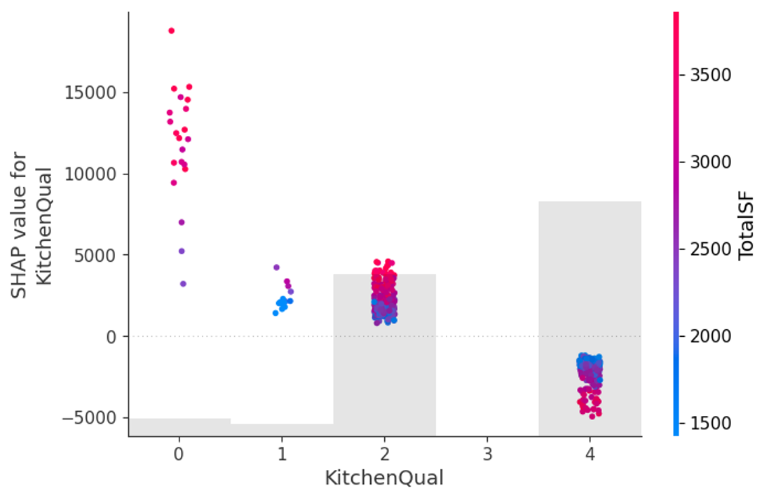
SHAP values can give finer-grained information about the impact of features. The chart below shows the impact of kitchen quality on sales price with coloration added to reflect the size of the house corresponding to each observation. We can clearly see that there is a clustering effect, in which smaller houses remain closer to 0 and larger houses take more extreme values in both directions. This indicates that the quality of a kitchen has a stronger effect, whether it be positive or negative, on the sales price in larger houses. Thus, all things (and especially the cost of a renovation) being equal, a kitchen renovation in a larger house will yield a higher profit than a kitchen renovation in a smaller house. In the next section, we give average dollar amounts for this difference.

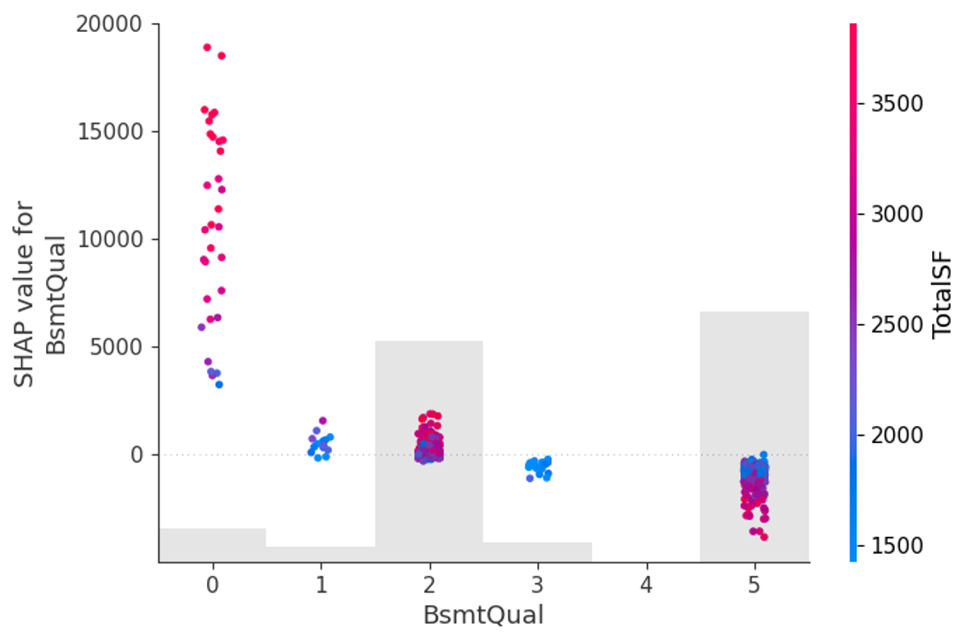
Similar interactions between the size of a house and the SHAP values of features were found for basement quality and number of bathrooms. The relevant charts reflecting the clustering effects are provided below, and the average increased profit of renovating larger houses are given in the next section. We investigated interactions between the SHAP values of the mutable features and other features besides the houses’ square footage, but no strong effects were found.


Flipper Recommendations
Our findings can be summarized in the below tables.
Total Bathrooms: For a larger than average home, adding a half-bath to a home with two total bathrooms added $9,429 to the home value on average. For a smaller than average home, this added $6,629 on average.

Basement Quality: For a larger than average home, upgrading the basement quality from typical to good added $2,081 to the home value on average. For a smaller than average home, this added $851 on average.

Kitchen Quality: For a larger than average home, upgrading the kitchen quality from typical to good added $5,472 to the home value on average. For a smaller than average home, this added $3,163 on average.

Our final recommendations for a flipper are to focus on homes with:
- a typical or poor kitchen
- 2 bathrooms or less
- a typical or poor basement
- 2,500 sq ft or larger
- low value in high value neighborhoods
And to perform one of the following three renovations, with consideration for the expense of undertaking the renovation, which was not included in this study:
- Increase number of bathrooms from 2 to 2.5 (potential value increase of ~$8,000)
- Upgrade basement quality from typical to good (potential value increase of ~$1,500)
- Upgrade kitchen quality from typical to good (potential value increase of ~$4,500)
Code for this project is available on GitHub.

