Rate Hikes or not? Developing a machine learning model to predict Fed interest rate decisions
Low interest rates have been part of the Federal Reserve’s monetary policy since 2007 when they were put in place for the post-recession recovery effort. At the end of 2015, the Fed decided on a rate hike for the first time since the crisis and it is expected to continue raising rates multiple times in 2017.
However, the Federal Open Market Committee (FOMC) doesn’t always follow market expectations when it makes its decisions, which can cause huge global capital market volatility. It is valuable to foresee the fed's action and make use of the stock market volatility. So the big question : According to the US economic data, Is it possible to build a model to predict the interest rate and the Fed's action?
Why is the interest rate important?
The interest rate in an economy not only reflects, but influences economic activities.
If the interest rates is too high, people can't afford the price of loans to invest in new equipment, new houses, and new employees.
Conversely, if the interest is too low, there is huge risk of overheating the economy, which will cause bubbles (for example in the stock market) or the inflation that happens in a lot of developing countries now, where prices go up as a result of too much money chasing too few goods.
How can we avoid the market volatility?
Usually, the Fed tries to balance economic activity and inflation, pushing the jobless rate as low as possible while also ensuring that prices don’t rise too quickly or too high. The question is: Is there any other impact factors that influence Fed's decision? What kind of model does the Fed use to predict whether the interest rates should change?
Assuming the Fed makes the decision on the US economic data, I scraped 100+ of the most popular US economic data ( .csv files) from "https://fred.stlouisfed.org" with Python (Scrapy and Selenium).
What kinds of machine learning models can we choose?
In order to answer the questions above, two kinds of models could be considered :
- Linear Regression (numeric change in interest rates)
- Classification (Fed's action)
The linear regression model can predict the interest rate based on US economic activities. Meanwhile, the classification model can predict the Fed's action (0 means no change, 1 stands for increase, -1 for decrease).
Feature Selection
Most of the variables could be removed for several reasons:
- Variables with very low correlation to the interest rate, such as the GDP of CHINA.
- Variables dependent on the interest rate, such as the yield of bond, LIBOR in London, one or ten years Treasury Bill rate.
- Variables with high multicollinearity such as Unemployment Level, Employed population rate, Light vehicle sales, Employee payrolls, the labor force participation rate, and New Housing permits.
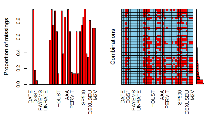
- Variables only existing annually as this kind of variable create a lot of missing value (Figure 1), also the monthly data is more reasonable and explicit to describe the Fed's decisions on interest rates.
 Figure 1 shows annual data creates many missing values
Feature Engineering
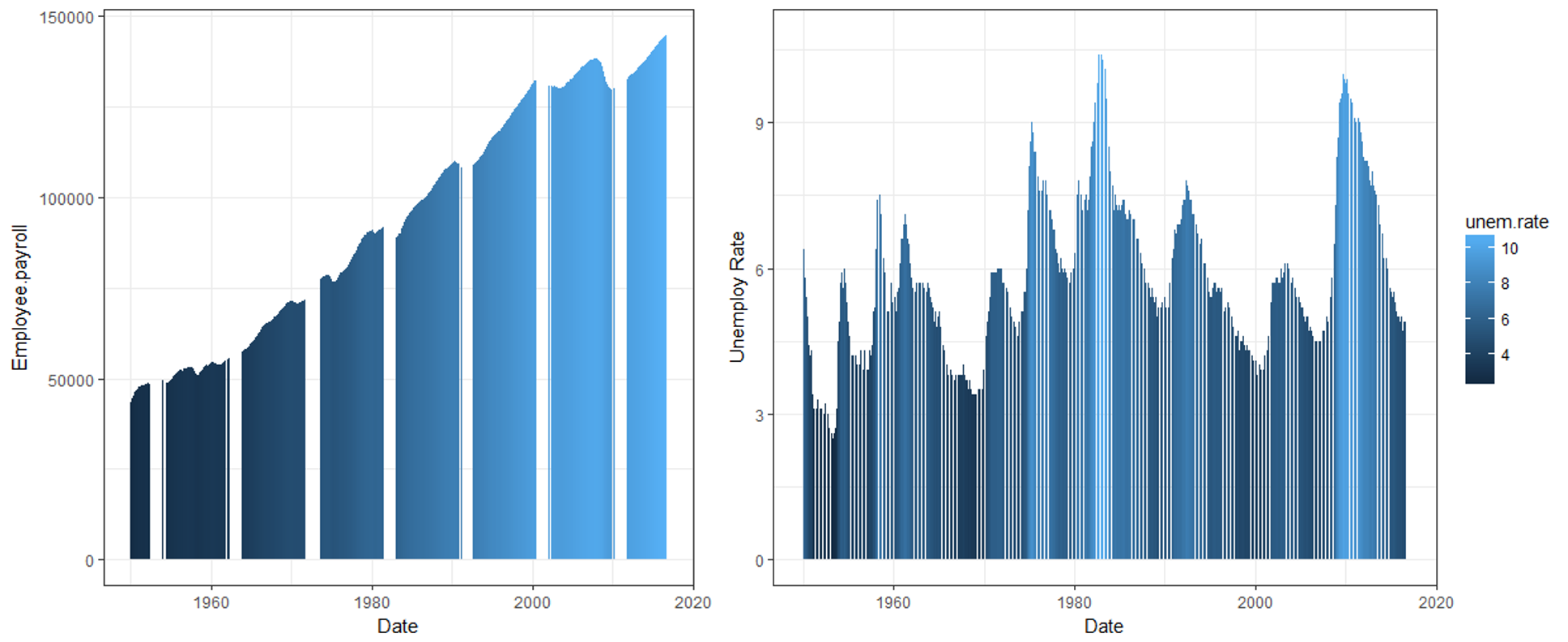
The interest rate is kind of oscillating variable that ranged from 0-20%, so all the variables changing over time should be transformed to oscillating variables.
The change rate was used to replace the number (right part of figure above)
Linear Regression Model
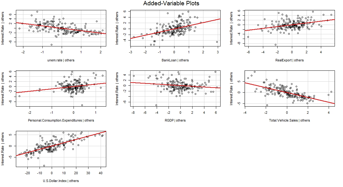
After feature engineering, the linear regression model was built to predict the interest rate, and 7 variables were significant.
Interest.Rate =13.092 + 1.101 * BL
+ 0.390 * RE
+ 0.148 * US.Dollar.Index
+ 0.930 * P.C.E
- 1.036 * UE
- 0.136 * RGDP
- 1.090 * T.V.S
where
BL is the bank loan rate, when bank loans increase, the interest rate should be raised to reduce the risk of bubbles and inflation;
RE is the real export rate, while the Real Export rate grows faster, more money flows into the market, and the Fed should raise the interest rate to withdraw the extra export earned.
US.Dollar.Index stands for the value of US dollar, the more expensive the dollar is, the higher risk of overheating the economic, and the higher possibility the Fed raise the interest rate.
P.C.E is the personal consumption expenditures rate. The rate of consumption increase, which always caused by prices going up faster. The Fed could raise the interest rate to avoid inflation.
UE is the unemployed rate. The higher the unemployment rate, the lower interest rates are required to encourage the investment.
RGDP is the rate of GDP growth. The higher the rate of GDP growth, the more money is required in the market for the economy to function. If real GDP grows too quickly, the Fed could reduce the interest rate to lower the price of loans and lower risk of deflation.
T.V.S is the total vehicle sales. Vehicle sales relate to mortgages, which means more and more vehicle sales require the lower the price of loans (decreasing the interest rate).
The statistic of the model is below:
The added variable plots above shows the contribution of each additional variable. Distinct patterns are indications of good contributions to the linear model.
Regression Diagnostic
In order to evaluate the assumption of the linear regression, four diagnostic plots (below) were brought up. The upper left plot shows the residuals (the vertical distance from a point to the regression line) versus the fitted values. Note that three points are numbered 667, 373, and 706, which does not necessarily indicate a problem but does mean we need to pay special attention to them.
The upper right plot is a Normal Q-Q plot of the residuals. Recall that one of the assumptions of a least-squares regression is that the errors are normally distributed. This plot evaluates that assumption. Here, three points 667, 373, and 706 lie pretty far from the dashed line, especially the point 706 indicate large deviation from the line.
The lower left plot is identical to the upper left plot. The only difference is the square root of the standardized residuals on the y-axis, which the residuals are re-scaled so that they have a mean of zero and a variance of one. This plot eliminates the sign on the residual, with large residuals (both positive and negative) plotting at the top and small residuals plotting at the bottom. The red line shows the trend and the variance in the residuals shouldn't change as a function of x, which means the red line should be relatively flat. It is here, except at the far left end, where several points with near zero or negative fit values pull the line down, and points 373 and 706 at the right end pull the trend up.
The lower right plot shows the standardized residuals against leverage. Leverage reflects both the distance from the center and the isolation of a point. The plot also contours values of Cook’s distance, which measures how much the regression would change if a point was deleted. Cook’s distance increases due to large leverage and residuals. If one point far from the center with a large residual can severely affect the regression. On this plot, point 706 has a large Cook's distance (>0.5), and point 622 with large leverage has a big Cook's distance but still smaller than 0.5.
Investigate the outliers and leverage points
As a result of the regression diagnostic, four data point with larger residue or greater leverage need further investigated, which happened in 1981-01-01, 2001-10-01, 2005-07-01, and 2008-10-01. From the table below, we can see large difference between the real interest rate and the prediction. What happened at those times? -- Economic Recession possibly caused by the wrong interest rate decision by Fed!
1981-01-01:The Fed kept the real interest rate too high, which caused economic recession. "The early 1980s recession in the United States began in July 1981 and ended in November 1982. One cause was the Federal Reserve's contractionary monetary policy, which sought to rein in the high inflation. In the wake of the 1973 oil crisis and the 1979 energy crisis, stagflation began to afflict the economy."
2001-10-01: From 2000 to 2001, the Federal Reserve, in a move to protect the economy from the overvalued stock market, made successive interest rate increases, but after September 11, 2001 attacking the economy need lower interest rate to reduce the cost of investment and rebuilt. As the result of Fed kept the interest rate higher, the severe, prolonged recession occurred in United States in 2002 and 2003.
2005-07-01: In 2001, Alan Greenspan dropped interest rates to a low 1% in order to jump the economy after the ".com" bubble, comparing with the model that show the real interest kept too low, which indicated the housing bubble in 2005-2006. In order to rein the housing bubble, the Fed started rate hiking with too fast steps from 2005, which caused U.S economy slowed sharply at the end of 2005. Also, as the real interest rate is too high, the mortgage and credit crisis occurred in 2007.
2008-10-01 (the only data point with the Cook's distance >0.5): Since the advent of the global financial crisis of 2007–08 and since the risk-free short-term nominal interest rates were either at or close to zero, a policy termed 'quantitative easing' (QE) have been used by the United States, the United Kingdom, and the Eurozone. QE is essentially a new way of raising the money supply in the economy. Since interest rates have been near zero, the whole world has had trouble using just monetary policy to jump out of the great recession.
Also from the figure below, comparing the prediction and the real interest rate over 40 years, we can find the model distorted after 2008. Due to the irregular QE, QE2, and QE3 and the material negative interest rate, the real interest rate has trouble reflecting the economy, which is abnormal in history, with bubble in stock market, but lower inflation and economic recession.
Should the outlier and leverage points be removed for the model?
If the points with large residue or great leverage were removed, the R-squared value would increase by almost 0.1, which means a great improvement on the model. Meanwhile, this would then easily point out these major policy events.
How about the prediction on the points removed?
The new model point out the larger singularity between the prediction and the real interest rate, which can foresee the crisis while the gap beyond one threshold.
Classification
Now the linear model can help predict the value of the interest rate, which can foresee and direct the Fed's decision.
Can we directly predict if the Fed take an action on the interest rate?
Random Tree
Data were trained with best mtry=2, but due to the unbalance of the data in each class, large error occurred in the classes "increase" and "decrease".
Neural Network
As the selected feature without multicollinearity, multinomial log-linear models via neural networks was used to predict the Fed's decision.
How the Fed will deal with the interest rate in the coming December's FOMC meeting?
From the linear model and figure above, we see the gap between the prediction and real interest rate, which reveals the potential raise of the interest rate.
but both the random forest and the neural network predict higher possible that the Fed will keep the current interest rate.
Conclusion:
The Fed has many economists making very advanced models about the economy. For this project, I wanted to see if looking at a few basic features could model past Fed actions. The main features made intuitive sense, but I would still trust the Fed’s econometric modeling processes to determine how to change a metric as important as interest rates going forward.


